Beginner’s Guide to Simple Linear Regression

Welcome to the Beginner’s Guide to Simple Linear Regression—a key starting point in the world of Machine Learning. If you’re new to this field, don’t worry. We’re here to make things easy and fun.

So, what’s linear regression? It’s basically a tool we use to understand relationships between different things. Think of it as the ABC of supervised learning, where we predict outcomes based on input data.

In this guide, we’ll break down linear regression into simple bits, showing you why it’s important and how it opens doors to more advanced stuff. You’ll learn the basics, see it in action, and be ready to tackle real-world problems. Get ready for an exciting journey that will boost your skills and change how you view data science. Let’s dive in and unravel the linear regression!

Section 1: Understanding Linear Regression

Simple linear regression is a method to predict a dependent variable’s value based on the value of an independent variable. It finds the best-fit straight line through the data points. It has the following components:

• Dependent Variable (y): The outcome you’re trying to predict.
• Independent Variable (x): The input you think affects the dependent variable.
• Linear Equation (y = mx + c): The formula to find the predicted value of y for any x.
  • y: Dependent variable.
  • x: Independent variable.
  • m: Slope of the line, indicating the change in y for a one-unit change in x.
  • c: y-intercept, the value of y when x is 0.

Simple linear regression looks for the linear relationship between x and y, using the equation to predict future values of y based on new inputs of x. It’s foundational in understanding how variables are related and is used across many fields for prediction.

Section 2: The Mathematics Behind Linear Regression

Linear regression is all about finding the best line that fits your data. This line, called the regression line, shows the relationship between two variables: the one you’re predicting (Y) and the one you’re using to make predictions (X). The equation is described by the following:

\[ Y = mX + c \]

\(Y\) is what we’re predicting, \(X\) is what we’re using to predict, \(m\) is the slope (showing the direction of the relationship), and \(c\) is where the line hits the Y-axis.

Cost Function

A key component in linear regression is the cost function, also known as the loss or error function. This function measures how well our regression line predicts the actual data points. One common cost function used in linear regression is the Mean Squared Error (MSE), which calculates the average of the squares of the errors between the predicted and actual values.

The formula for MSE is given by:

\[ MSE = \frac{1}{n} \sum_{i=1}^{n} (Y_i – \hat{Y}_i)^2 \]

Where:

• \(n\) is the number of data points,
• \(Y_i\) is the actual value of the dependent variable for the ith data point,
• \(\hat{Y}_i\) is the predicted value for the ith data point.

The goal in linear regression is to minimize the cost function, meaning we want our predicted values (\(\hat{Y}\)) to be as close as possible to the actual values (\(Y\)). 

Gradient Descent

To achieve this goal of minimizing the cost function, we use an optimization algorithm known as gradient descent. Gradient descent helps us adjust the parameters of our linear equation (\(m\) and \(c\)) to find the minimum possible value of the cost function. Think of it as descending down a hill until the lowest point is reached; that lowest point represents the minimum error or cost.

Gradient descent iteratively adjusts \(m\) and \(c\) by taking the negative of the gradient (or the slope) of the cost function at the current point. By repeatedly taking small steps in the direction of the steepest decrease, we eventually reach the minimum value.

Section 3: Preparing Jupyter Notebook & Python

Python is a versatile programming language that’s become the lingua franca for data science due to its simplicity and the vast ecosystem of data science libraries available. Jupyter Notebook on the other hand is an open-source web application that allows you to create and share documents containing live code, equations, visualizations, and narrative text. Here’s how to get started:

Step 1. Install Python: Visit the official Python website and download the latest version of Python. During installation, ensure that you check the option to “Add Python to PATH” to make Python accessible from the command line.

Step 2. Install Jupyter Notebook: The easiest way to install Jupyter Notebook is via Python’s package manager, pip. Open your command line (Command Prompt on Windows, Terminal on macOS and Linux) and run the following command:

  pip install notebook

This command downloads and installs Jupyter Notebook and its dependencies.

Step 3. Launch Jupyter Notebook: After installation, you can start Jupyter Notebook by running the following command in your command line:

  jupyter notebook

This command will open Jupyter Notebook in your default web browser, showing a dashboard where you can create new notebooks or open existing ones.

Section 4: Implementing Linear Regression in Python

For our example, we’ll use a simplified dataset related to housing prices, with two main features: the size of the house (in square feet) and the price of the house (in thousands of dollars). Our goal is to predict the price of a house based on its size. This dataset is fictional but serves well to illustrate the concept of linear regression.

Data Preprocessing

Before we can build our model, we need to prepare our dataset. This process, known as data preprocessing, involves several steps to ensure our data is clean and ready for analysis. 

1. Handling Missing Values: Datasets in the real world often come with missing values. We can handle these by removing the rows with missing values or replacing them with a summary statistic (like the mean or median).
2. Encoding Categorical Data: Our current dataset doesn’t include categorical data, but if it did, we would need to convert these categories into numerical values. This process is known as encoding.
3. Feature Scaling: While not always necessary for linear regression, feature scaling can be important in other types of models. It involves standardizing the range of our features to ensure that no single feature dominates due to its scale.

For the sake of simplicity, we’ll assume our dataset is clean and doesn’t require encoding or feature scaling.

Exploratory Data Analysis (EDA)

EDA is a critical step in data science, allowing us to understand the relationships between variables. Let’s visualize our dataset using Matplotlib to see the relationship between house size and price.

import pandas as pd
import matplotlib.pyplot as plt

# Sample dataset
data = {
    'Size': [650, 785, 1200, 495, 945, 1175],
    'Price': [300, 350, 500, 250, 400, 475]
}

df = pd.DataFrame(data)

# Plotting the dataset
plt.figure(figsize=(10, 6))
plt.scatter(df['Size'], df['Price'], color='blue')
plt.title('House Size vs Price')
plt.xlabel('Size (sqft)')
plt.ylabel('Price (in thousands)')
plt.grid(True)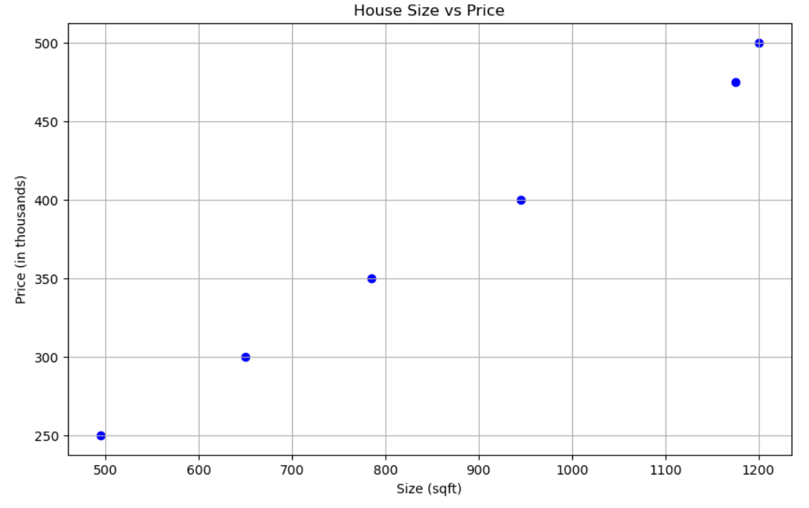
plt.show()

This code snippet creates a scatter plot of our dataset. You should see a positive correlation between the size of the house and its price, indicating that as the size increases, the price tends to increase as well.

Building the Linear Regression Model

Now, let’s use Python’s `scikit-learn` library to build and train our linear regression model.

from sklearn.model_selection import train_test_split
from sklearn.linear_model import LinearRegression

# Preparing the data

X = df['Size'].values.reshape(-1,1)  # Feature matrix
y = df['Price'].values  # Target variable

# Splitting the dataset into training and testing sets
X_train, X_test, y_train, y_test = train_test_split(X, y, test_size=0.2, random_state=42)

# Creating a linear regression model
model = LinearRegression()

# Training the model
model.fit(X_train, y_train)

# Predicting the prices
predictions = model.predict(X_test)

# Displaying the coefficient and intercept
print("Coefficient (m):", model.coef_[0])
print("Intercept (c):", model.intercept_)

# Plotting the regression line
plt.figure(figsize=(10, 6))
plt.scatter(df['Size'], df['Price'], color='blue')  # Original data points
plt.plot(X, model.predict(X), color='red')  # Regression line
plt.title('House Size vs Price (with Regression Line)')
plt.xlabel('Size (sqft)')
plt.ylabel('Price (in thousands)')
plt.grid(True)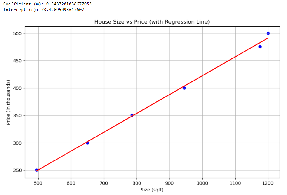
plt.show()

This code trains a linear regression model on our dataset, splitting it into training and testing sets to evaluate its performance. The `LinearRegression` model from `scikit-learn` is straightforward to use and provides us with the coefficients of our linear equation, allowing us to understand the relationship between size and price quantitatively.

Section 5: Beyond Simple Linear Regression

Having mastered simple linear regression, you’re now ready to explore more complex models that can handle a broader range of real-world scenarios. This chapter introduces multiple linear regression, a natural extension of the concepts you’ve learned, and discusses methods for dealing with non-linear relationships.

Multiple Linear Regression

Simple linear regression is powerful for predicting an outcome based on a single predictor variable. However, in the real world, outcomes are often influenced by multiple factors. Multiple linear regression extends simple linear regression to include several independent variables, offering a more comprehensive model for prediction.

The equation for multiple linear regression is an extension of the simple linear equation:

\[ Y = b_0 + b_1X_1 + b_2X_2 + … + b_nX_n + \epsilon \]

Here, \(Y\) represents the dependent variable you’re trying to predict, \(X_1, X_2, …, X_n\) are the independent variables, \(b_1, b_2, …, b_n\) are the coefficients for each independent variable, \(b_0\) is the y-intercept, and \(\epsilon\) is the error term.

Multiple linear regression allows us to understand how each independent variable contributes to the dependent variable while controlling for the presence of other independent variables. This model is implemented similarly to simple linear regression in `scikit-learn`, with the main difference being the inclusion of multiple features in your feature matrix \(X\).

Dealing with Non-linearity

Not all relationships between independent and dependent variables are linear. Sometimes, the relationship might be polynomial or follow another non-linear pattern. When linear regression models are not sufficient due to non-linear data patterns, you can use several approaches to capture these relationships:

• Polynomial Regression: This is a form of regression analysis where the relationship between the independent variable \(x\) and the dependent variable \(y\) is modeled as an nth degree polynomial. Polynomial regression fits a nonlinear relationship between the value of \(x\) and the corresponding conditional mean of \(y\), denoted \(E(y|x)\).
• Transformation of Variables: Applying transformations to your variables can sometimes turn a non-linear relationship into a linear one. Common transformations include taking the logarithm, square root, or power of one or more variables.
• Non-linear Models: Beyond transforming variables or using polynomial regression, you might explore entirely non-linear models better suited to your data. Examples include decision trees, k-nearest neighbors (KNN), and neural networks, each offering different approaches to modeling complex relationships.

Section 6: Tips for Further Learning

Embarking on a journey in machine learning and data science can be as thrilling as it is challenging. This final chapter aims to equip you with strategies to navigate the learning curve efficiently, overcome information overload, bridge skill gaps, and manage your time effectively. These tips are designed to support your continuous learning and growth in the field.

Overcoming Information Overload

The abundance of resources available can sometimes feel overwhelming. Here’s how to navigate through:

• Curate Your Resources: Start with foundational books or courses recommended by reputable sources. Look for content created by well-known professionals in the field. In fact, I learned linear regression through YT videos, Wikipedia, and some books. 
• Limit Your Sources: Rather than jumping between dozens of resources, choose a few comprehensive ones and stick with them until you’ve grasped the basics.
• Practical Application: Theory is essential, but practice solidifies learning. Work on projects or problems as you learn to apply new concepts.

Bridging Skill Gaps

Supplementary learning in mathematics, statistics, and programming is crucial for your growth in machine learning.

• Mathematics and Statistics: Before you dive into machine learning, it’s imperative to assess yourself if you have a solid background in math and statistics. If you don’t have any, websites like Khan Academy and Coursera offer free courses in calculus, linear algebra, probability, and statistics—fundamental concepts in machine learning.
• Programming: If you’re new to Python, start with introductory programming courses. Codecademy, Udemy, and freeCodeCamp are excellent platforms to learn Python basics and beyond. Simplilearn also offers some free introductory courses not just in Python, but data science libraries as well such as NumPy, Panda, Matplotlib, Scikit Learn, Keras, and Tensorflow. 
• Specialized Courses: Once you have a handle on the basics, enroll in specialized machine learning and data science courses. Look for courses that offer hands-on projects.

Time Management Advice

Balancing learning with professional and personal responsibilities requires effective time management.

• Set Realistic Goals: Define clear, achievable goals for your learning. Breaking down your learning objectives into smaller, manageable tasks can make them seem less daunting.
• Dedicated Study Time: Allocate specific times of the day or week for learning. Consistency is key to making progress. As for me, I study machine learning every day after work, for about 90 minutes from Monday to Friday. It’s up to you to find the right time to study and practice, depending on your priorities. 
• Apply What You Learn: Integrate your new knowledge into your professional work if possible. It’s an excellent way to reinforce learning and demonstrate value to your employer.
• Join a Community: Engaging with a community of learners can provide motivation and support. Look for online forums, study groups, or local meetups.

Embrace the Journey

Remember, the journey into machine learning is a marathon, not a sprint. Patience, persistence, and a positive attitude are your best allies. Learning something new, especially a field as vast and dynamic as machine learning, is a process filled with challenges and rewards. Celebrate your progress, however small, and stay curious. The field of machine learning is evolving rapidly, and there’s always something new to discover.

By following these tips and continuously seeking knowledge, you’ll not only advance your skills but also open doors to new opportunities and innovations in the field of machine learning. Welcome to an exciting journey of lifelong learning and discovery.

Conclusion

Throughout this guide, we’ve explored simple linear regression, a fundamental concept in machine learning. We covered everything from basics to practical implementation in Python, aiming to kickstart your journey into data science.

We addressed common challenges faced by beginners and emphasized the importance of quality learning resources. Through hands-on examples, you learned how to build your first linear regression model and expand into more complex analyses.

But this is just the beginning. Machine learning is vast, and there’s much more to explore beyond linear regression. I encourage you to keep learning, experimenting, and sharing your journey with others.

Thank you for joining me on this adventure. May your passion for learning lead you to new heights in your career and personal growth. Keep exploring and enjoy the journey ahead in the world of machine learning!

FAQs