Beginner’s Guide to Polynomial Regression

Polynomial regression is a form of regression analysis in which the relationship between the independent variable \(x\) and the dependent variable \(y\) is modeled as an \(n\)th degree polynomial. Polynomial regression fits a nonlinear relationship between the value of \(x\) and the corresponding conditional mean of \(y\), denoted \(E(y|x)\). This regression algorithm has been used to describe nonlinear phenomena such as the growth rate of tissues, the distribution of carbon isotopes in lake sediments, and the progression of disease epidemics.

By the end of this guide, you’ll grasp the basics of polynomial regression and appreciate its role in crafting intelligent, data-driven solutions in machine learning projects. Let’s dive in and demystify polynomial regression, making it an accessible and practical tool in your data science toolkit.

Section 1: Conceptual Understanding

Regression analysis is a statistical method used to understand the relationship between dependent (target) and independent (predictor) variables. Its primary goal is to predict the outcome of a dependent variable based on the known values of independent variables. This technique is crucial for identifying trends, making forecasts, and decision-making in various fields, from finance to healthcare.

Linear vs. Polynomial Regression

• Linear Regression is the starting point for most predictive modeling tasks. It assumes a straight-line (linear) relationship between the dependent and independent variables. Simple and straightforward, it’s used when the data appears to follow a linear trend.
• Polynomial Regression, on the other hand, extends linear regression by introducing powers of the independent variable. This approach is used when the relationship between the variables is curvilinear, allowing you to model a wider range of phenomena. The model fits a polynomial equation to the data, which can better handle complexities and nuances in datasets.

When to Use Polynomial Regression

Polynomial regression is your go-to when you observe a non-linear pattern in your data plots. If a linear model fails to capture the underlying trends or if you suspect that the effect of an independent variable on the dependent variable changes at different levels of that variable, polynomial regression can provide a more accurate and nuanced model. 

Polynomial regression is particularly useful in cases where the strength and direction of the relationship between variables vary, or when dealing with phenomena that inherently follow a non-linear progression.

While linear regression offers simplicity and ease of interpretation, polynomial regression brings flexibility and the ability to model more complex relationships. Knowing when to apply each is a crucial skill in data science, allowing for more accurate predictions and insights.

Section 2: The Math Behind Polynomial Regression

Polynomial regression models the relationship between the independent variable \(x\) and the dependent variable \(y\) as an \(n\)th degree polynomial in \(x\). The general formula for a polynomial regression of degree \(n\) is:

\[ y = \beta_0 + \beta_1x + \beta_2x^2 + \beta_3x^3 + \ldots + \beta_nx^n + \epsilon \]

Here, 

• \(y\) represents the dependent variable we’re trying to predict, 
• \(x\) is the independent variable, 
• \(\beta_0\) is the y-intercept of the curve, indicating where it crosses the y-axis. 
• \(\beta_1, \beta_2, \ldots, \beta_n\) are the coefficients that determine the shape and direction of the polynomial curve. By adjusting these values, the model can fit more complex datasets. 
• Degree (\(n\)): The highest power of \(x\) in the polynomial, determining the curve’s complexity. A higher degree can model more complex relationships but also risks overfitting. 
• \(\epsilon\) is the error term that represents the difference between the observed and predicted values, highlighting the model’s accuracy.

Why Use Polynomial Regression?

Polynomial regression is chosen over linear regression for several reasons:

1. Modeling Non-linear Relationships: Many real-world relationships between variables are not linear. Polynomial regression can capture these complex patterns effectively.
2. Flexibility: The ability to adjust the degree of the polynomial allows for fine-tuning the model’s complexity based on the dataset’s intricacies.
3. Improved Accuracy: By better capturing the nuances in the data, polynomial regression often yields more accurate predictions for datasets with non-linear trends.

Use Cases of Polynomial Regression

Polynomial regression shines in scenarios where the relationship between variables is known to be non-linear. Some common applications include:

• Economic Growth: Modeling GDP growth rates based on various economic factors.
• Biological Sciences: Understanding growth rates of organisms or chemical reaction rates under different conditions.
• Market Research: Predicting sales growth based on advertising spend.

Section 3: Implementing Polynomial Regression

Python’s scikit-learn library simplifies implementing polynomial regression. Follow these steps to apply it to your dataset. For this one, I will analyze the aqueous solubility of inorganic compounds at various temperatures. 

1. Import Necessary Libraries

import numpy as np
import pandas as pd
from sklearn.model_selection import train_test_split
from sklearn.preprocessing import PolynomialFeatures
from sklearn.linear_model import LinearRegression
from sklearn.metrics import mean_squared_error, r2_score
import matplotlib.pyplot as plt

2. Load Your Dataset

For this example, I manually input the data for temperature (in C) and solubility for various inorganic salts. I got the data from the Solubility Data Series of the International Union of Pure and Applied Chemistry. If you have a .csv or .xlsx sheet for your data, you can use a pandas function like pd.read_csv. Here’s the code I used to manually enter the data:

data = {
    'Temperature (C)': [0,10,20,25,30,40,50,60,70,80,90,100],
    'Solubility': [26.28,26.32,26.41,26.45,26.52,26.67,26.84,27.03,27.25,27.50,27.78,28.05]
}

solubility = pd.DataFrame(data)
solubility

3. Prepare the Data

Split your dataset into the independent variable \(X\) and dependent variable \(y\). Also, split the data into training and testing sets.

# Separating into independent (X) and dependent (y) variables
X = solubility[['Temperature (C)']]
y = solubility['Solubility']

4. Transform Data for Polynomial Features

# Generating polynomial features
degree = 2  # You can adjust the degree as needed
poly_features = PolynomialFeatures(degree=degree)
X_poly = poly_features.fit_transform(X)

5. Train the Model

# Creating the regression model and fitting it to the polynomial data
model = LinearRegression()
model.fit(X_poly, y)

6. Make Predictions

# Predictions using the model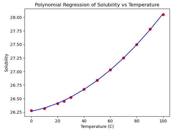
y_pred = model.predict(X_poly)

7. Visualize the Results

Plot the original data points and the polynomial regression curve.

# Plotting the results
plt.scatter(X, y, color='red')  # Original data points
plt.plot(X, y_pred, color='blue')  # Regression line
plt.title('Polynomial Regression of Solubility vs Temperature')
plt.xlabel('Temperature (C)')
plt.ylabel('Solubility')
plt.show()

Here’s the result of the model:

8. Analyzing and Interpreting Results

Evaluating the performance of your polynomial regression model involves several metrics:

• Mean Squared Error (MSE): Measures the average of the squares of the errors between observed and predicted values. Lower values indicate better fit.
• Coefficient of Determination (\(R^2\) Score): Indicates the proportion of the variance in the dependent variable predictable from the independent variable(s).

# Calculating Mean Squared Error (MSE) and R-squared (R2) for the model
mse = mean_squared_error(y, y_pred)
r2 = r2_score(y, y_pred)
mse, r2

The results I got for MSE is 9.377184649196335e-05 while for \(R^2\) is 0.9997153469029614. 

An \(R^2\) score closer to 1 indicates a better model fit. However, be cautious of overfitting, especially with high-degree polynomials. Balancing model complexity with predictive accuracy is key to effective polynomial regression.

This practical guide provides the fundamentals to get started with polynomial regression in Python. With practice and exploration, you’ll gain confidence in applying this technique to various data science challenges.

Section 4: Applying Polynomial Regression to Real-World Problems

Polynomial regression offers a versatile tool for tackling a wide range of real-world problems where the relationship between variables isn’t linear. Understanding its application can significantly impact your problem-solving approach in data science projects.

1. Predicting Energy Consumption: In the utilities sector, energy consumption patterns can be complex. Polynomial regression can model the non-linear relationship between temperature and energy usage, helping predict peak energy demands.
2. Real Estate Pricing Models: Real estate prices are influenced by numerous factors in a non-linear manner. Polynomial regression can help in creating more accurate pricing models by considering the non-linear effects of variables like location, area, and the number of rooms on price.
3. E-commerce Sales Forecasting: The relationship between advertising spend and sales revenue is often non-linear, with diminishing returns after a point. Polynomial regression can model these trends, helping e-commerce businesses optimize their marketing budgets for maximum ROI.

Tips for Approaching Problem-Solving with Polynomial Regression

• Start with Exploratory Data Analysis (EDA): Before jumping into polynomial regression, visually explore your data to understand its structure, detect outliers, and identify potential non-linear relationships.
• Select the Right Degree: The degree of the polynomial is crucial. Too low, and you risk underfitting; too high, and your model may overfit. Cross-validation can help in selecting an optimal degree by evaluating model performance on unseen data.
• Feature Scaling: When working with polynomial features, especially of higher degrees, feature scaling becomes essential to prevent numerical computation issues and improve model training efficiency.
• Regularization: Consider regularization techniques (like Ridge or Lasso) to control overfitting by penalizing large coefficients in higher-degree polynomial models.
• Validate Model Performance: Always use a hold-out validation set or cross-validation to assess your model’s performance. This step helps ensure that your model generalizes well to new, unseen data.
• Iterative Approach: Polynomial regression, like many machine learning techniques, benefits from an iterative approach. Start simple, evaluate, and then gradually increase complexity as needed, based on model performance and business objectives.

Applying polynomial regression effectively requires a blend of technical skills and domain knowledge. By understanding the nuances of your data and the specific challenges of your problem domain, you can leverage polynomial regression to uncover insights and make predictions that linear models might miss, driving value and innovation in your projects.

Key Takeaways

Polynomial regression offers a robust method for modeling and understanding complex, non-linear relationships in data. Its versatility and power facilitate deeper insights and more accurate predictions, especially in scenarios where traditional linear models fall short. This knowledge not only enhances your analytical capabilities but also serves as a springboard to the broader domain of predictive modeling and data science.

As you continue your journey, let the principles of polynomial regression inspire you to explore further. The realm of machine learning is rich with techniques and methodologies waiting to be discovered and applied. Each new model or algorithm you learn not only broadens your skill set but also opens up new avenues for innovation and problem-solving in real-world scenarios.

Remember, the field of machine learning is as challenging as it is rewarding. Your curiosity, willingness to experiment, and commitment to continuous learning are your most valuable assets. Embrace the complexities, celebrate the successes, and learn from the setbacks. The path from beginner to expert is a journey of a thousand steps, and each step forward, no matter how small, is a victory in its own right.

So, armed with the knowledge of polynomial regression and an eagerness to delve deeper, step forth into the ever-evolving world of machine learning. Whether it’s through personal projects, professional endeavors, or academic pursuits, the opportunity to apply your skills to solve real-world problems is immense. Let your curiosity guide you, and never stop learning, for the future of data science is bright, and it awaits your contribution.