Beginner’s Guide to Multiple Linear Regression

Welcome to our Beginner’s Guide to Multiple Linear Regression, your gateway to understanding a key concept in machine learning. Multiple linear regression helps predict outcomes by analyzing the relationship between one dependent variable and multiple independent variables, making it an essential skill for data scientists. 

This guide simplifies the complexities of this statistical technique, tailored for beginners eager to apply it in real-world scenarios, like consumer behavior analysis or housing price forecasts. Through clear explanations and Python examples, I’ll help you grasp multiple linear regression and its role in supervised learning. Dive into this concise yet comprehensive guide to enhance your machine learning journey, one insightful step at a time.

Section 1: Understanding Multiple Linear Regression

Imagine you’re trying to predict the final grade of students in a class. You might initially think that the number of hours they study is the only factor. But in reality, their performance could also depend on several other factors like attendance, participation, and even the amount of sleep they get. This is where multiple linear regression comes into play. It’s like a multi-tool that considers various factors (variables) to predict an outcome accurately.

Multiple linear regression (MLR) is a statistical method that allows us to examine how multiple independent variables are related to one dependent variable. Think of the independent variables as the different ingredients in a recipe, and the dependent variable as the final dish you’re trying to cook. MLR helps us understand how each ingredient changes the taste of the dish and predicts what happens to the dish if we adjust the amount of one or more ingredients.

Simple vs. Multiple Linear Regression

The difference between simple and multiple linear regression is essentially the number of predictors used. Simple linear regression uses just one predictor (ingredient) to predict an outcome. It’s like predicting the sweetness of a cake based only on the amount of sugar you add. 

Multiple linear regression, on the other hand, uses two or more predictors. It’s like predicting the sweetness of the cake based on the amount of sugar, the type of flour, and the amount of baking powder you use.

Key Concepts and Terminology

• Dependent Variable: This is what you’re trying to predict or explain. In our student grade example, the final grade would be the dependent variable.
• Independent Variables: These are the factors you think may affect the dependent variable. In the same example, hours of study, attendance, and sleep are independent variables.
• Coefficients: These are numbers that represent the relationship between each independent variable and the dependent variable. If the coefficient is positive, it means that as the independent variable increases, the dependent variable also increases. A negative coefficient means the opposite.

Section 2: The Mathematics Behind Multiple Linear Regression

At the heart of multiple linear regression is the idea that we can predict the value of a dependent variable (let’s call it \(Y\)) based on the values of several independent variables (\(X_1, X_2, …, X_n\)). The relationship between \(Y\) and each \(X_i\) is linear, meaning it can be represented by a straight line. This line is like a trend line that best fits our data points.

The equation for multiple linear regression might look a bit complex at first, but it’s an extension of the simple linear regression equation, \(Y = a + bX\), where:

• \(Y\) is still our dependent variable we want to predict,
• \(a\) is the intercept,
• \(b_1, b_2, …, b_n\) are the coefficients for each independent variable (\(X_1, X_2, …, X_n\)), representing how much \(Y\) changes with a unit change in each \(X_i\),
• \(\epsilon\) is the error term, accounting for the difference between the predicted and actual values (it’s what makes our line a “best fit” rather than a perfect fit).

In multiple linear regression, we have more than one independent variable, so the equation expands to:

\[ Y = a + b_1X_1 + b_2X_2 + … + b_nX_n + \epsilon \]

Section 3: Preparing Your Environment

Before diving into the practical application of multiple linear regression, it’s essential to set up a working environment where you can write and test your code. Python, along with Jupyter Notebooks, provides a powerful and interactive platform for data analysis and machine learning. Let’s get started by setting up Python and Jupyter Notebooks, followed by an introduction to some of the key libraries you’ll use for multiple linear regression.

Install Python: If you haven’t already, download and install Python from the official Python website. Make sure to download a version that’s 3.x, as it’s the most up-to-date and compatible with the libraries we’ll be using.

Install Jupyter Notebooks: Jupyter Notebooks offer an interactive coding environment that allows you to write and execute Python code in a web browser. It’s perfect for data analysis and visualization. You can install Jupyter via pip (Python’s package installer) by running the following command in your terminal or command prompt:

Pip install notebook

Launch Jupyter Notebooks: Once installed, you can launch Jupyter Notebooks by running the command `jupyter notebook` in your terminal or command prompt. This command will open Jupyter in your default web browser, ready for you to start coding.

Recommended Libraries for Multiple Linear Regression

For multiple linear regression in Python, several libraries make the process smoother and more efficient. Here’s a brief overview of each:

• NumPy: A fundamental package for numerical computation in Python. It provides support for arrays, mathematical functions, and matrix operations, which are crucial for handling data and calculations in regression analysis.
  • Installation command: `pip install numpy`
• Pandas: An essential library for data manipulation and analysis. It offers data structures and operations for manipulating numerical tables and time series, making it easier to handle and preprocess your dataset.
  • Installation command: `pip install pandas`
• Matplotlib: A plotting library for Python that allows you to create a wide variety of static, animated, and interactive visualizations. It’s useful for plotting graphs to visualize your data and regression results.
  • Installation command: `pip install matplotlib`
• scikit-learn: A simple and efficient tool for data mining and data analysis built on NumPy, SciPy, and matplotlib. It includes support for various machine learning models, including linear regression, making it a go-to library for predictive data analysis.
  • Installation command: `pip install scikit-learn`

Section 4: Conducting Multiple Linear Regression in Python

Conducting multiple linear regression in Python is a straightforward process once you have your environment set up. In this section, we’ll walk through the steps to perform multiple linear regression using a Jupyter Notebook. We’ll use a hypothetical dataset that contains various independent variables (like hours of study, class attendance, etc.) to predict a dependent variable (final grade).

Step 1: Data Collection and Preparation

First, we need a dataset. For simplicity, let’s assume we have a dataset called `landprice1.csv` that contains area and distance as independent variables to determine the price of land, our dependent variable. 

import pandas as pd

# Load the dataset
dataset = pd.read_csv('C:\\Users\\Martin\\OneDrive\\landprice1.csv')

# Preview the data
dataset.head()

Step 2: Splitting the Dataset into Training and Testing Sets

We split our data into a training set (to train our model) and a test set (to evaluate its performance).

from sklearn.model_selection import train_test_split

X = dataset[["Area", "Distance"]].valuesY = dataset["Price"].values
X_train, X_test, Y_train, Y_test = train_test_split(X, Y, test_size=0.4, random_state=0)

Step 3: Building the Multiple Linear Regression Model

Now, let’s build our multiple linear regression model using scikit-learn.

from sklearn.metrics import mean_squared_error, r2_score
from sklearn.model_selection import train_test_split
from sklearn.linear_model import LinearRegression
import numpy as np

# Initialize the model
model = LinearRegression()

# Fit the model to the training data
model.fit(X_train, Y_train)

Step 4: Training the Model with the Training Set

Training the model involves finding the best coefficients for our independent variables. This step is accomplished by the `.fit()` method we just called.

Y_pred = model.predict(X_test)

Step 5: Evaluating the Model’s Performance on the Test Set

After training, we evaluate the model’s performance on the test set to see how well it predicts new, unseen data.

from sklearn.metrics import mean_squared_error, r2_score

print('Coefficients: \n', model.coef_)
print('Y intercept: \n', model.intercept_)
print('Mean Squared Error: %.2f' % mean_squared_error(Y_test, Y_pred))
print('Coefficient of determination: %.2f' % r2_score(Y_test, Y_pred))

Step 6: Visualizing the Results

To get a better grasp of how land area and distance affects land price, we can plot it using matplolib. 

import matplotlib.pyplot as plt
import numpy as np

X1 = dataset["Area"]
X2 = dataset["Distance"]
X3 = dataset["Crime Rate"]
Y = dataset["Price"]

# Calculate R-squared values
r2_area = np.corrcoef(X1, Y)[0, 1] ** 2
r2_distance = np.corrcoef(X2, Y)[0, 1] ** 2
r2_crime_rate = np.corrcoef(X3, Y)[0, 1] ** 2

# Calculate the best fit lines
m1, b1 = np.polyfit(X1, Y, 1)
m2, b2 = np.polyfit(X2, Y, 1)
m3, b3 = np.polyfit(X3, Y, 1)

plt.figure(figsize = (10,4))
plt.suptitle("Multiple Linear Regression Models", fontsize = 20)

# Area vs Price
plt.subplot(1,3,1)
plt.scatter(X1, Y)
plt.plot(X1, m1*X1 + b1, color='pink')  # Best fit line
plt.title(f"Area of the Lot vs Price\nR² = {r2_area:.2f}")

# Distance vs Price
plt.subplot(1,3,2)
plt.scatter(X2, Y)
plt.plot(X2, m2*X2 + b2, color='pink')  # Best fit line
plt.title(f"Distance vs Price\nR² = {r2_distance:.2f}")

# Crime Rate vs Price
plt.subplot(1,3,3)
plt.scatter(X3, Y)
plt.plot(X3, m3*X3 + b3, color='pink')  # Best fit line
plt.title(f"Crime Rate vs Price\nR² = {r2_crime_rate:.2f}")

plt.tight_layout()
plt.show()

plt.tight_layout()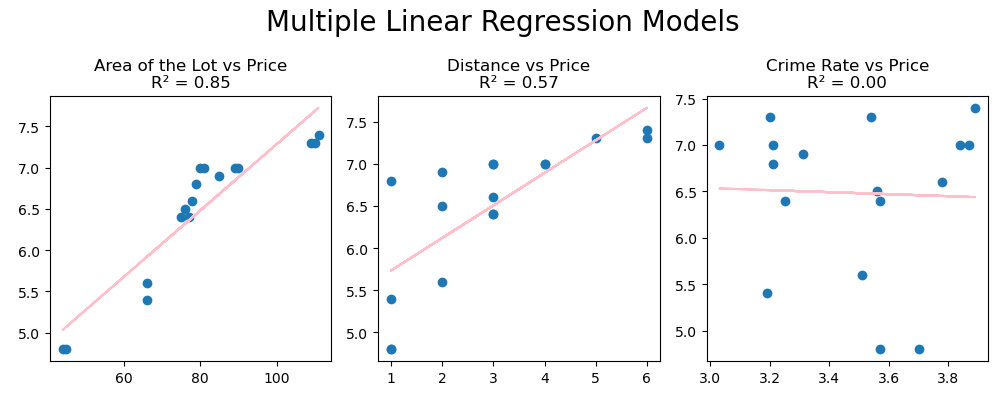

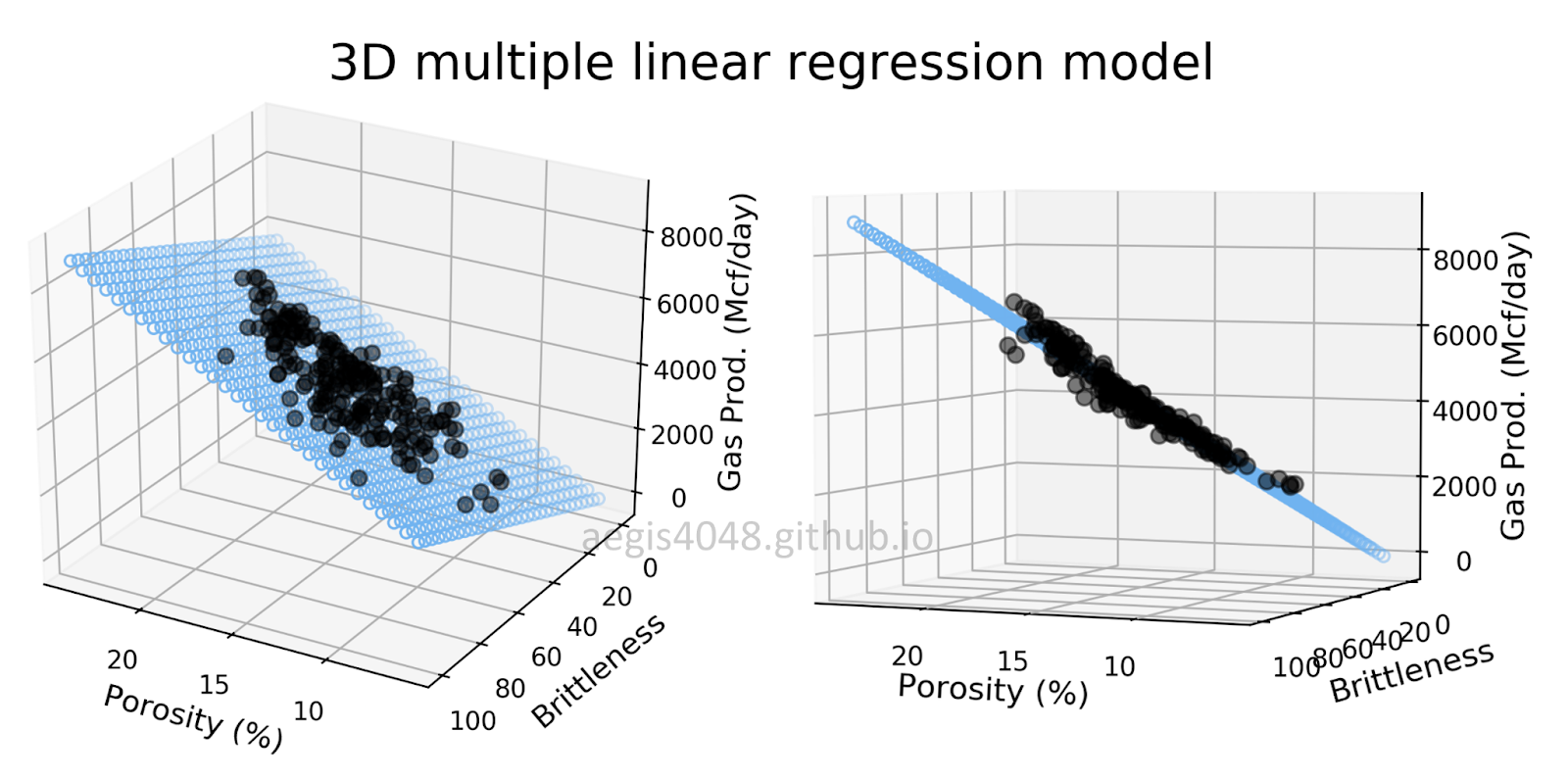
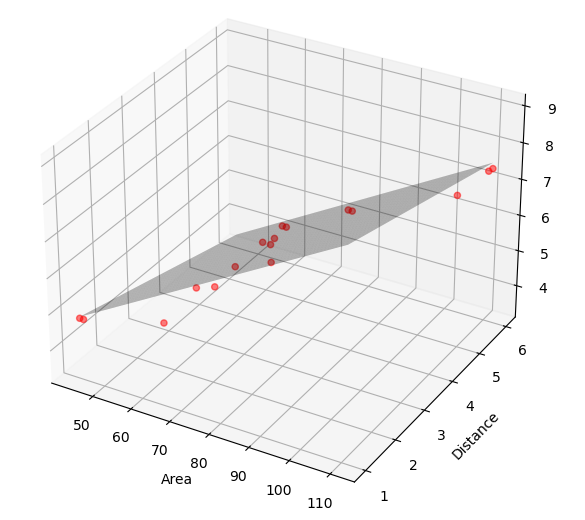
Here are the plots for bivariate regression. This means we only plotted one independent variable against one dependent variable to see how they’re correlated. We’re doing this to see if the independent variables have a linear relationship with the dependent variable. In cases where the regression line is curved, we’ll use polynomial regression. If we want to see it in 3D, we can use the code below. 

# Create a mesh grid of values to plot the plane.
x_surf, y_surf = np.meshgrid(np.linspace(X[:, 0].min(), X[:, 0].max(), 100),
                            np.linspace(X[:, 1].min(), X[:, 1].max(), 100))
# Flatten the mesh grid to pass into predict to get corresponding Z values
onlyX = pd.DataFrame({'Area': x_surf.ravel(), 'Distance': y_surf.ravel()})
fittedY = model.predict(onlyX)

# Convert the predicted result in an array
Z = fittedY.reshape(x_surf.shape)

# Plotting
fig = plt.figure(figsize=(10, 7))
ax = fig.add_subplot(111, projection='3d')

# Scatter plot for actual data
ax.scatter(X[:, 0], X[:, 1], Y, color='red', marker='o', alpha=0.5)
# Plotting the surface plane
ax.plot_surface(x_surf, y_surf, Z, color='None', alpha=0.3)

# Set labels and titles
ax.set_xlabel('Area')
ax.set_ylabel('Distance')
ax.set_zlabel('Price')
ax.set_title('Multiple Linear Regression Model')

# Show plot
plt.show()

Here’s how the plot looks like.

Step 7: Interpreting the Results

• The Mean Squared Error (MSE) measures the average of the squares of the errors, i.e., the average squared difference between the estimated values and the actual value. A lower MSE indicates a better fit.
• The \(R^2\) Score represents the proportion of the variance for the dependent variable that’s predicted from the independent variables. It ranges from 0 to 1, with 1 indicating perfect predictions.
• Interpreting these metrics helps us understand the model’s accuracy and effectiveness in making predictions. For instance, a high R^2 score close to 1 means our model does a great job in predicting the final grade based on the given independent variables.

Through these steps, you’ve now completed a cycle of conducting multiple linear regression in Python. From preparing your data to interpreting your model’s performance, each step is crucial in the journey of predictive modeling and data science.

Section 5: Key Considerations in Multiple Linear Regression

Multiple linear regression is a powerful tool for predictive analysis and data science. However, it operates under several assumptions. Understanding these assumptions, how to check for their violations, and remedying these violations are crucial to ensure the reliability and accuracy of your model. Additionally, there are strategies to improve model accuracy that you can employ throughout the analysis process.

Assumptions of Multiple Linear Regression Analysis

1. Linearity: The relationship between the independent variables and the dependent variable is linear.
2. Independence: Observations are independent of each other.
3. Homoscedasticity: The variance of error terms (residuals) is constant across all levels of the independent variables.
4. Normality: The residuals of the model are normally distributed.
5. No multicollinearity: Independent variables are not too highly correlated with each other.

Checking and Remedying Violations

• Linearity: You can check linearity by plotting each independent variable against the dependent variable. If the plots show curved patterns, linearity is violated. Transforming the variables or adding polynomial terms can help.
• Independence: This is more of a study design issue. Ensure your data collection method doesn’t introduce dependency.
• Homoscedasticity: Plot the residuals against the predicted values. If the spread of residuals is uneven, it indicates heteroscedasticity. Using transformations (like log transformation) or adopting a different modeling approach can help.
• Normality: A Q-Q plot of the residuals can help assess this. If residuals deviate significantly from the line, consider using transformations or robust regression methods.
• No multicollinearity: Check correlations among independent variables. High correlations suggest multicollinearity. Variable selection, principal component analysis (PCA), or ridge regression can mitigate this.

Tips for Improving Model Accuracy

• Feature Engineering: Creating new features or modifying existing ones can provide new insights and improve model accuracy.
• Feature Selection: Not all variables are useful. Use techniques like backward elimination, forward selection, or regularization methods (LASSO, Ridge) to select relevant variables.
• Data Quality: Ensuring high-quality data is crucial. Handle missing data appropriately, and remove or correct outliers.
• Cross-validation: Use cross-validation techniques to assess how your model will generalize to an independent dataset.
• Regularization: Techniques like LASSO and Ridge can prevent overfitting by penalizing large coefficients.
• Model Tuning: Adjusting model parameters can significantly impact performance. Grid search or random search methods can automate the search for the best parameters.

Conclusion

Throughout this comprehensive guide, we’ve journeyed from the foundational concepts of multiple linear regression to the practical steps of conducting analyses in Python, and even touched upon advanced topics for further exploration. As we wrap up, let’s recap the key takeaways and look ahead to how you can continue to grow and apply your newfound knowledge.

• Multiple Linear Regression is a powerful statistical technique that models the relationship between one dependent variable and two or more independent variables, offering insights into how various factors influence outcomes.
• Preparation and Understanding of your data through exploratory data analysis (EDA) are crucial steps before diving into regression analysis. This ensures that the assumptions of multiple linear regression are met and that the data is clean and ready for modeling.
• Implementation in Python is made accessible through libraries such as NumPy, Pandas, Matplotlib, and scikit-learn, which together provide a robust toolkit for data manipulation, visualization, and model building.
• Model Evaluation involves understanding the metrics like R-squared and Mean Squared Error (MSE) to assess the accuracy and effectiveness of your regression model.

Machine learning is a vast and dynamic field, with multiple linear regression being just the starting point. As you grow more comfortable with these concepts, we encourage you to explore more advanced topics such as logistic regression for classification problems, decision trees, random forests, support vector machines, and neural networks. Each of these techniques offers unique perspectives and tools for tackling complex analytical challenges.

Remember, the journey into machine learning is one of continuous learning and curiosity. The field is constantly evolving, with new algorithms, tools, and best practices emerging. Stay engaged with the community, keep experimenting, and never stop learning.

Thank you for embarking on this journey with us through the Beginner’s Guide to Multiple Linear Regression. We hope it has sparked a passion for data science and machine learning that will drive you to further explore, learn, and innovate in this exciting field.

Frequently Asked Questions