Linear Models: A Comprehensive Guide

This guide is all about linear models in machine learning, a key starting point for anyone new to the field. Linear models are essential for understanding supervised learning and are used widely for prediction and analysis. We’ll cover the basics, including different types of linear models and how they work. This guide aims to make learning about linear models straightforward and clear, helping you build a strong foundation in machine learning. Let’s dive into it together.

Section 1: Basics of Linear Models

Linear models predict or explain a dependent variable (\(y\)) using a linear combination of one or more independent variables (\(x_1, x_2, …, x_n\)). The formula below shows how each predictor (\(x_i\)) is weighted by a coefficient (\(\beta_i\)), with \(\beta_0\) as the y-intercept and \(\epsilon\) representing error not explained by the model.

\[y = \beta_0 + \beta_1x_1 + \beta_2x_2 + … + \beta_nx_n + \epsilon\]

The Linear Equation

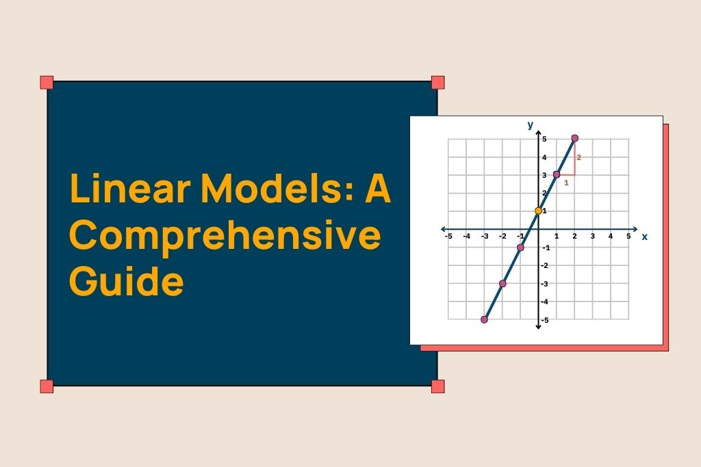
Linear models are built from linear equations. These equations allow us to predict the value of the dependent variable based on the values of the independent variables. The simplest form of a linear equation in two dimensions (one independent variable) is:

\[ y = \beta_0 + \beta_1x \]

This equation represents a straight line where \( \beta_0 \) is the intercept (the value of \( y \) when \( x \) is 0) and \( \beta_1 \) is the slope of the line (the change in \( y \) for a one-unit change in \( x \)).

The Least Squares Method

The method of least squares determines the best-fitting line through a set of points. It does so by minimizing the sum of the squares of the differences (residuals) between the observed values and the values predicted by the linear model. Mathematically, it solves the following optimization problem:

\[ \min_{\beta_0, \beta_1,…,\beta_n} \ \sum_{i=1}^{N} (y_i – (\beta_0 + \beta_1x_{1i} + … + \beta_nx_{ni}))^2 \]

Here, \( N \) is the number of observations, and \( y_i \) and \( x_{1i}, …, x_{ni} \) are the observed values of the dependent and independent variables, respectively.

Assumptions Behind Linear Models

For linear models to provide reliable predictions and insights, certain assumptions about the data must be met, including:

1. Linearity: The relationship between the independent and dependent variables should be linear.
2. Independence: Observations should be independent of each other.
3. Homoscedasticity: The variance of the error terms should be constant across all levels of the independent variables.
4. Normal Distribution of Errors: The error terms should be normally distributed.

In the next sections, we’ll explore how these assumptions of linear models are applied in various scenarios, and how they contribute to the field of supervised learning. Understanding these basics sets the stage for delving deeper into more complex models and their applications in real-world problems.

Section 2: Types of Linear Models

Linear models, in their various forms, serve as versatile tools for statistical analysis and prediction. Here, we’ll explore some of the key types of linear models, each with its unique characteristics and applications.

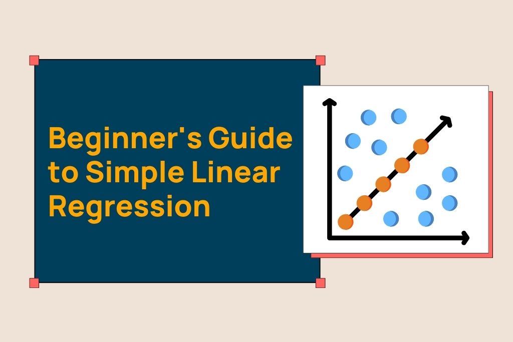
Simple Linear Regression

Simple linear regression is the most basic form of linear models, involving a single independent variable. It models the relationship between two variables by fitting a linear equation to observed data. The equation of a simple linear regression model is:

\[ y = \beta_0 + \beta_1x + \epsilon \]

Where \( y \) is the dependent variable, \( x \) is the independent variable, \( \beta_0 \) is the y-intercept, \( \beta_1 \) is the slope of the line, and \( \epsilon \) represents the error term. This model assumes a straight-line relationship between the dependent and independent variables.

Multiple Linear Regression

Multiple linear regression extends simple linear regression by including two or more independent variables. It is used to understand the relationship between one dependent variable and several independent variables. The model is represented as:

\[ y = \beta_0 + \beta_1x_1 + \beta_2x_2 + … + \beta_nx_n + \epsilon \]

This model allows for more complex analyses and can provide insights into how different independent variables impact the dependent variable together and individually.

Generalized Linear Models

Generalized linear models (GLMs) extend linear models to allow the dependent variable to have a non-normal distribution. They are a flexible generalization of ordinary linear regression that allows for response variables to have error distribution models other than a normal distribution. 

GLMs consist of three components: a linear predictor, a link function, and a variance function. The general form of a GLM is:

\[ g(E(y)) = \beta_0 + \beta_1x_1 + … + \beta_nx_n \]

Where \( g() \) is the link function that defines the relationship between the linear predictor and the mean of the distribution function.

Linear Mixed Models

Linear mixed models (LMMs) are an extension of simple linear models for data that are collected and summarized in groups. These models are particularly useful for data with multiple levels of random effects, like nested or hierarchical data.

In LMMs, fixed effects (generalizable to the entire population) and random effects (specific to the groups) are included. The model can be represented as:

\[ y = X\beta + Z\gamma + \epsilon \]

Where \( X \) and \( Z \) are known design matrices, \( \beta \) are fixed effects, \( \gamma \) are random effects, and \( \epsilon \) is the error term.

Log Linear Models

A log-linear model is a type of math model where the logarithm of a function equals a straight sum of its parameters. This setup lets us use linear regression, even with multiple variables.

\[ exp\left( c+\sum_i w_i f_i(X) \right) \]

This model is used to explore the relationship between categorical variables, often analyzing the frequency of occurrences that fall into categories defined by two or more variables.

Section 3: Linear Models in Supervised Learning

Linear models play a pivotal role in the realm of supervised learning, a branch of machine learning focused on learning a function that maps an input to an output based on example input-output pairs. In this context, linear models are valued for their simplicity, interpretability, and efficiency.

1. Foundation for Understanding: Linear models are often the starting point for learning about supervised machine learning. They provide a straightforward way to understand the basic principles of machine learning, such as feature importance, overfitting, underfitting, and model evaluation.
2. Interpretability: One of the significant advantages of linear models is their interpretability. They make it easy to understand the relationship between input features and the target output, which is crucial in many applications, especially in domains like finance, healthcare, and social sciences, where understanding the decision-making process is as important as the decision itself.
3. Benchmarking: In supervised learning, linear models often serve as a benchmark for more complex models. Due to their simplicity, they are quick to implement and provide a baseline level of performance against which other more complex models can be compared.
4. High-Dimensional Spaces: Linear models are particularly effective in high-dimensional spaces where the number of features is large compared to the number of samples. Techniques like regularization in linear regression (Lasso, Ridge) are designed to handle such situations effectively, preventing overfitting and aiding in feature selection.

Section 4: Implementing Linear Models

Implementing linear models involves a series of systematic steps, from data preparation to model evaluation. Here, I’ll provide a step-by-step guide to building a linear model, along with common challenges and their solutions.

Step 1. Define the Problem

Clearly understand and define the objective of your model. Are you predicting a continuous variable (regression) or classifying data into categories (classification)?

Step 2. Data Collection

Gather the required data. This data can come from various sources like databases, CSV files, or APIs.

Step 3. Data Preprocessing

• Clean the data: Handle missing values, remove duplicates, and deal with outliers.
• Feature engineering: Create new features from existing data if necessary.
• Data transformation: Normalize or standardize your data, especially for features with varying scales.
• Split the data into training and testing sets to evaluate the model’s performance later.

Step 4. Selecting the Model

Choose a linear model based on your problem definition. For example, use linear regression for predicting values or logistic regression for classification tasks.

Step 5. Train the Model

Use the training dataset to train the model. This involves finding the coefficients (parameters) that best fit the training data.

For linear regression, this typically involves finding the least squares estimates of the coefficients.

Step 6. Model Evaluation

Evaluate the model’s performance using the test data.

Use appropriate metrics like Mean Squared Error (MSE) for regression or accuracy and ROC curves for classification.

Step 7. Model Optimization

Fine-tune the model. This may involve feature selection, regularization (like Lasso or Ridge), or hyperparameter tuning.

Step 8. Deployment

Once the model performs satisfactorily, deploy it for real-world use. This could be in a production environment, a web application, etc.

Step 9. Monitoring and Updating

Continuously monitor the model’s performance and update it as needed. Data drift or changes in external factors may necessitate retraining or modifications.

Common Challenges and Solutions

1. Overfitting:  Use regularization techniques, simplify the model, or increase training data.
2. Underfitting: Add more features, increase model complexity, or use a different model.
3. Multicollinearity: Identify and remove highly correlated independent variables, or use dimensionality reduction techniques.
4. Non-linearity: Include polynomial or interaction terms, or consider using non-linear models.
5. Heteroscedasticity (non-constant variance): Transform the dependent variable or use weighted least squares.
6. Missing Data: Impute missing values or use models that handle missing data effectively.
7. Bias in Data: Collect more diverse and representative data, or apply techniques to balance the data.
8. Scalability with Large Datasets: Optimize code, use algorithms designed for large datasets, or leverage cloud computing resources.

Section 5: Advancing with Linear Models

As you grow more comfortable with the basics of linear models, there are various strategies and advanced techniques you can employ to enhance model accuracy and efficiency. These tips and techniques can help you extract more value from your linear modeling efforts.

Tips for Improving Model Accuracy and Efficiency

1. Feature Engineering: Improving the quality and relevance of input features can significantly enhance model performance. This includes creating new features from existing data, selecting relevant features, and transforming variables for better model fit.
2. Data Quality: Ensure the data is clean, accurate, and representative. Handle missing values appropriately, remove outliers, or use robust methods that can handle outliers.
3. Regularization: Employ regularization techniques like Lasso (L1 regularization) and Ridge (L2 regularization) to prevent overfitting, especially when dealing with high-dimensional data.
4. Cross-Validation: Use cross-validation techniques to assess the model’s performance. This helps in understanding how the model generalizes to an independent dataset and in tuning hyperparameters.
5. Model Updating: Regularly update your model with new data to keep it relevant. Models can become outdated as underlying data distributions change over time.
6. Scalability and Performance Optimization: For large datasets, optimize your code, use efficient libraries, and leverage parallel computing or distributed processing when necessary.
7. Interpretability and Explainability: Focus on making your model interpretable. This is especially important in fields where understanding the decision-making process is crucial, like in healthcare or finance.

Advanced Techniques in Linear Modeling

1. Polynomial and Interaction Terms: Incorporate polynomial or interaction terms in your model to capture non-linear relationships between variables.
2. Elastic Net Regularization: This technique combines L1 and L2 regularization and can yield better results than using either regularization technique alone.
3. Generalized Additive Models (GAMs): These models extend linear models by allowing non-linear relationships between the dependent and independent variables, providing greater flexibility.
4. Quantile Regression: Instead of predicting a mean value, quantile regression predicts a quantile, which can be useful for understanding the variability in data.
5. Mixed-Effects Models: Useful in scenarios where data is collected from hierarchical or nested experiments. These models account for both fixed and random effects.
6. Dimensionality Reduction Techniques: Techniques like Principal Component Analysis (PCA) can be used to reduce the number of input variables, simplifying the model without significant loss of information.
7. Robust Regression: For data with outliers, robust regression techniques are more appropriate as they are less sensitive to outliers compared to ordinary least squares.
8. Machine Learning Pipelines: Incorporate linear models into larger machine learning pipelines for tasks like feature preprocessing, dimensionality reduction, and ensemble modeling.
9. Time Series Analysis: Advanced time series techniques, like ARIMA or Vector Autoregression (VAR), can be used for more accurate forecasting in data with temporal dependencies.
10. Integration with Deep Learning: In some complex scenarios, linear models can be integrated with deep learning approaches, combining the interpretability of linear models with the power of neural networks.

Section 6: Tools and Resources for Linear Modeling

To effectively implement and advance your skills in linear modeling, having access to the right tools and educational resources is crucial. Below are some recommended software, libraries, books, and online courses that can enhance your knowledge and proficiency in linear modeling.

Software and Libraries for Linear Modeling

• R and R Studio: R is a statistical programming language with excellent packages for linear modeling such as `lm` for linear regression and `lme4` for mixed-effects models.
• Python: Python is a versatile programming language with libraries like `scikit-learn` for linear regression, logistic regression, and more, and `statsmodels` for more detailed statistical modeling.
• MATLAB: MATLAB is a high-level language and interactive environment that is particularly strong in matrix operations, making it suitable for linear modeling.
• SAS: SAS is a software suite for advanced analytics that also offers robust capabilities for linear modeling.
• Excel: For simpler linear modeling tasks, Microsoft Excel can be used, especially with its Data Analysis Toolpak.
• Julia: Julia, a high-performance programming language for technical computing, has packages for linear models and is gaining popularity for its speed.

Recommended Books

1. “An Introduction to Statistical Learning” by Gareth James, Daniela Witten, Trevor Hastie, and Robert Tibshirani: This book provides a broad and accessible overview of linear modeling with practical examples.
2. “The Elements of Statistical Learning” by Trevor Hastie, Robert Tibshirani, and Jerome Friedman: A more advanced text than the previous, offering in-depth insights into linear models and other statistical learning methods.
3. “Applied Linear Statistical Models” by Michael H. Kutner, Christopher J. Nachtsheim, John Neter, and William Li: This comprehensive text covers a wide range of linear modeling techniques with practical applications.
4. “Linear Models with R” by Julian J. Faraway: Specifically focused on linear models using R, this book is great for those who prefer a hands-on approach.

Conclusion

Linear models are crucial in supervised learning and provide a solid foundation for understanding machine learning. They’re straightforward, easy to interpret, and widely applicable across industries. While mastering linear models is a great starting point, remember that the field of data science is always evolving. Keep exploring, learning, and experimenting with more complex techniques to unlock new possibilities. Stay curious, persistent, and enjoy the journey of discovery in the world of machine learning.