Beginner’s Guide to LASSO Regression

LASSO Regression, short for Least Absolute Shrinkage and Selection Operator, is a method of linear regression that incorporates a regularization term. This technique is highly regarded in the data science community, especially in areas like machine learning, for its dual capacity to carry out variable selection and regularization. These features significantly improve the prediction accuracy and interpretability of the statistical model produced.

To explore LASSO Regression further, we will explore how it differentiates itself from other regression models by its unique ability to reduce the complexity of a model while maintaining accuracy. LASSO does this by penalizing the absolute size of the regression coefficients, effectively shrinking less important feature coefficients to zero. This results in models that are easier to interpret and often perform better on new, unseen data. 

In the upcoming sections, we will also discuss the mathematical foundation of LASSO Regression, its practical applications, and how to effectively implement it in python to achieve robust modeling results.

Section 1: Understanding LASSO Regression

LASSO Regression, also known as Least Absolute Shrinkage and Selection Operator, is a form of regularized linear regression. LASSO involves modifying the traditional least squares objective function by adding a penalty proportional to the absolute sum of the regression coefficients. The objective of LASSO Regression is to minimize the following function:

\[\min \left( \sum_{i=1}^{n} (y_i – \sum_{j=1}^{p} \beta_j x_{ij})^2 + \lambda \sum_{j=1}^{p} |\beta_j| \right)\]

Here, \(y_i\) represents the observed values of the response variable. The \(x_{ij}\) terms are the predictor variables, \(\beta_j\) are the coefficients of the model that need to be estimated, \(\lambda\) is the regularization parameter that controls the strength of the LASSO penalty, and \(n\) is the number of observations. 

To better illustrate how LASSO regression works, let’s have a conceptual example.

Imagine you are working on predicting house prices based on various features such as square footage, number of bedrooms, number of bathrooms, age of the house, and proximity to the city center. In a dataset with many features, some features may not significantly impact the price, or they may be redundant due to correlation with other features.

Using LASSO regression, you can both predict the house prices and identify which features are most important. Suppose you apply LASSO Regression to this dataset. The regularization term (controlled by \( \lambda \)) will penalize the coefficients of the less important features, driving them towards zero. This means LASSO might reduce the coefficients for features like “number of bathrooms” to zero if “number of bedrooms” already captures most of the variance needed to predict the house price, thus simplifying the model by automatically selecting more relevant features. 

This approach not only helps in building a model that avoids overfitting but also results in a model that is easier to interpret because it only includes significant features. For instance, if the final model includes only square footage and proximity to the city center, it suggests these are the primary drivers of house pricing in the dataset, providing clear insights into what factors most influence house prices.

Section 2: LASSO vs Ridge Regression

LASSO (Least Absolute Shrinkage and Selection Operator) and Ridge regression are both shrinkage methods and forms of regularized linear regressions that aim to prevent overfitting by introducing a penalty term to the loss function. Here’s how they differ:

Ridge Regression (L2 Norm)

• Penalty: Ridge Regression adds an L2 penalty to the regression model, which is the sum of the squares of the coefficients.
• Mathematical Formulation: If \(\beta\) represents the vector of coefficients, then the L2 penalty term is \(\lambda \sum_{j=1}^{p} \beta_j^2\), where \(\lambda\) is the regularization parameter.
• Effect: This penalty shrinks the coefficients but does not set any of them to zero, thus all features remain in the model but with reduced influence. It’s particularly useful when there is multicollinearity in the data or when the number of predictors is greater than the number of observations.
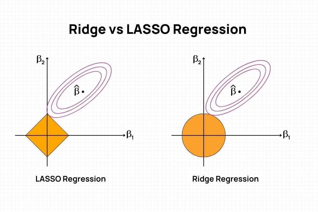
• Geometry: In a geometrical sense, Ridge Regression can be visualized as an elliptical contour that intersects with a circle (representing the L2 penalty) at the point of the minimized cost function.

LASSO Regression (L1 Norm)

• Penalty: LASSO (Least Absolute Shrinkage and Selection Operator) Regression involves an L1 penalty, which is the sum of the absolute values of the coefficients.
• Mathematical Formulation: The L1 penalty term is \(\lambda \sum_{j=1}^{p} |\beta_j|\)
• Effect: The L1 penalty can shrink some coefficients completely to zero, thus performing variable selection. LASSO is useful when you want a sparse model, i.e., a model with fewer parameters.
• Geometry: In a geometrical context, LASSO can be visualized as an elliptical contour intersecting with a diamond-shaped (rhombus) region (representing the L1 penalty) leading to coefficients being zeroed.

When to Use LASSO Regression

LASSO Regression is particularly suitable in certain situations due to its unique characteristics. Here’s some examples of when to use LASSO:

1. High Dimensionality: When you have a large number of features (predictors) in your dataset, especially when the number of features is close to or exceeds the number of observations, LASSO is very effective. In such cases, traditional regression techniques like Ordinary Least Squares (OLS) may overfit the data, but LASSO helps in reducing overfitting by penalizing the number of features included in the model.
2. Feature Selection: If your goal is to identify a subset of important predictors from a larger pool, LASSO is a great choice. Unlike other regression techniques that might retain most or all predictors, LASSO can shrink the coefficients of less important features to zero, effectively excluding them from the model. This leads to simpler, more interpretable models.
3. Multicollinearity: When predictors are highly correlated, OLS regression coefficients become unstable and their interpretation becomes difficult. LASSO can handle multicollinearity by penalizing the coefficients and potentially setting some of them to zero, which helps in reducing the variance without substantial increase in bias.
4. Predictive Accuracy: If improving the predictive accuracy of your model is a priority, especially in the presence of many features, LASSO can be a good choice. By reducing model complexity (through feature selection), it often improves the model’s out-of-sample prediction accuracy.
5. Interpretable Models: In scenarios where you need a model that’s easy to explain and understand, LASSO’s ability to produce sparser models (models with fewer parameters) is highly advantageous. This is particularly important in fields like medical research or social sciences, where explaining the role of each predictor is as important as the predictive accuracy of the model itself.

However, there are also situations where LASSO might not be the best choice. For example, if all features are known to be important, or if the number of observations is much smaller than the number of features, LASSO might overly simplify the model and exclude important predictors. Also, in cases with grouped predictors where you expect either all or none of the group members to be selected, techniques like Elastic Net, which combine LASSO and Ridge penalties, might be more suitable.

Section 3: Mathematical Intuition Behind LASSO Regression

The objective of LASSO regression is to minimize the sum of the squared residuals, similar to ordinary least squares (OLS), while also penalizing the absolute size of the regression coefficients. The penalty applied is proportional to the absolute value of the coefficients; this is where LASSO differs from Ridge Regression, which uses the square of coefficients as its penalty term. The LASSO regression equation can be represented as:

\[\min \left( \sum_{i=1}^{n} (y_i – \sum_{j=1}^{p} \beta_j x_{ij})^2 + \lambda \sum_{j=1}^{p} |\beta_j| \right)\]

The derivation of the LASSO regression equation involves understanding the balance between two main components: the least squares term and the LASSO penalty term.

• Least Square Terms: The least square terms, shown in the equation below, represents the sum of squared residuals. It measures the fit of the model to the data. The objective is to minimize these residuals, making the predicted values as close as possible to the actual values.

\[\sum_{i=1}^{n} (y_i – \sum_{j=1}^{p} \beta_j x_{ij})^2\]

• LASSO Penalty Term: The LASSO penalty term imposes a constraint on the sum of the absolute values of the coefficients. As \(\lambda\) increases, the penalty for having large coefficients increases. This penalty term encourages sparsity in the model coefficients, leading some coefficients to be exactly zero, effectively performing variable selection.

\[\lambda \sum_{j=1}^{p} |\beta_j|\]

The LASSO regression was derived by Robert Tibshirani in 1996 as a response to some of the limitations of ordinary least squares (OLS) regression in scenarios with high-dimensional data. In these cases, OLS can lead to overfitting and lack of interpretability. Tibshirani’s LASSO method aimed to address these issues by introducing a penalty term that encourages simpler, more interpretable models that generalize better to new data.

The choice of the absolute value of the coefficients for the penalty (as opposed to, say, the square of the coefficients, which is used in Ridge regression) is crucial. The absolute value function has a derivative that is not continuous at zero, which mathematically encourages coefficients to become exactly zero under optimization, thus achieving the goal of variable selection.

Section 4: Implementing LASSO Regression in Python

Implementing LASSO Regression in Python is straightforward with the help of libraries like scikit-learn, a powerful machine learning library. This section provides a step-by-step guide to applying LASSO Regression on a real-world dataset, highlighting key libraries and functions along the way.

Step 1: Importing Necessary Libraries

import pandas as pd
import numpy as np
from sklearn.linear_model import Lasso
from sklearn.model_selection import train_test_split
from sklearn.metrics import mean_squared_error
import matplotlib.pyplot as plt

Step 2: Loading and Preparing the Data

For this example, I’ll just create a synthetic dataset for determining house prices based on 3 variables/features: size, no. of bedrooms, and age. Then, let’s check the data first by calling the function pd.DataFrame() function.

# Create a synthetic dataset
data = {
    'Size': [1400, 2000, 2700, 1800, 1500, 2100, 2400, 2300, 1600, 3000],
    'Bedrooms': [2, 3, 4, 2, 3, 4, 3, 4, 2, 5],
    'Age': [5, 3, 8, 2, 4, 5, 7, 6, 3, 10],
    'Price': [250000, 315000, 350000, 280000, 265000, 330000, 295000, 320000, 260000, 380000]
}

df = pd.DataFrame(data)
# Display the first few rows of the dataframe

print(df.head())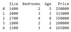

Step 3: Applying LASSO Regression and Training/Testing Data

# Splitting data into training and testing sets
X = df[['Size', 'Bedrooms', 'Age']]
y = df['Price']
X_train, X_test, y_train, y_test = train_test_split(X, y, test_size=0.2, random_state=42)

# Applying LASSO Regression
lasso = Lasso(alpha=1000) # alpha is the equivalent of lambda in LASSO formula
lasso.fit(X_train, y_train)

# Predicting and evaluating the model
y_pred = lasso.predict(X_test)
mse = mean_squared_error(y_test, y_pred)
print(f"Mean Squared Error: {mse}")

# Coefficients
print("Coefficients:", lasso.coef_)

The MSE for a \(\lambda\) value of 1000 is quite high. Let’s see when we adjust the \(\lambda\) to 100.

It slightly decreased since we put less penalty to some features. Finally, let’s see if the \(\lambda\) value is 10.

It seems that a \(\lambda\) value of 10 is our best choice since it gives the lowest MSE. However, in practice, selecting the best \(\lambda\) values must be done more systematically like using cross-validation, grid search, or domain knowledge.

Section 5: Practical Applications of LASSO Regression

LASSO regression has become an invaluable tool in the fields of chemistry and the sciences due to its ability to handle high-dimensional datasets and select relevant features, which is crucial for effective modeling and analysis. Here are some practical applications of LASSO regression in these domains:

Drug Discovery

In the pharmaceutical industry, LASSO regression can be used to identify key molecular descriptors that predict the biological activity of compounds. By reducing the dimensionality of the dataset and selecting only the most relevant features, LASSO helps in building predictive models for drug efficacy and safety, streamlining the drug discovery process by focusing on compounds most likely to succeed in later stages of development.

Spectral Data Analysis

Chemists use spectral data extensively for identifying substances and understanding molecular structures. LASSO can be applied to spectroscopic data (such as NMR, IR, or mass spectrometry data) to select the spectral features that are most informative for predicting properties of compounds or classifying different types of materials. This simplification is especially important in environments where the data is extremely high-dimensional, such as in metabolomics or proteomics.

Chemical Synthesis and Design

LASSO regression can help in the design of new chemicals by determining which features of chemical compounds are most important in achieving desired properties. This application is particularly valuable in materials science, where properties such as conductivity, reactivity, and strength are influenced by complex interactions between a large number of molecular variables.

Genomics and Bioinformatics

In genomics, LASSO regression is used for gene selection to identify which genes are most associated with certain diseases or traits. This is crucial in the development of personalized medicine and understanding genetic diseases. LASSO’s ability to handle the typically large datasets in genomics, where the number of predictors (genes) far exceeds the number of observations (patients), makes it particularly useful.

Quantitative Structure-Activity Relationship (QSAR) Modeling

QSAR modeling in cheminformatics involves predicting the activity or property of chemical compounds based on their molecular structure. LASSO regression helps in selecting meaningful molecular descriptors from a large pool, which significantly contributes to developing more accurate and interpretable QSAR models.

Through these applications, LASSO regression not only aids scientific discovery by providing a means to handle complex datasets efficiently but also improves the decision-making process by highlighting the most impactful factors in experimental outcomes.

Section 6: Optimizing Your LASSO Regression Model

Optimizing a LASSO Regression model involves fine-tuning several aspects, particularly selecting the right lambda (\(\lambda\)) value and implementing strategies for effective feature selection. By carefully addressing these aspects, one can enhance model performance significantly. Here are practical tips and strategies for optimizing your LASSO Regression model, along with advice on avoiding common pitfalls.

Tips for Selecting the Right Lambda Value

1. Cross-Validation: The most reliable method for choosing \(\lambda\) is through cross-validation, typically using a technique like k-fold cross-validation. Libraries such as `scikit-learn` provide functions like `LASSOCV`, which automatically perform cross-validation over a range of \(\lambda\) values to find the optimal one.
2. Grid Search: Implementing a grid search over a predefined range of \(\lambda\) values can also be effective. It involves training a LASSO model for each \(\lambda\) and selecting the value that minimizes the cross-validation error.
3. Balance Between Bias and Variance: Select a \(\lambda\) that achieves a good balance between underfitting (high bias) and overfitting (high variance). A very high \(\lambda\) can oversimplify the model (high bias), while a very low \(\lambda\) might lead to overfitting (low bias but high variance).
4. Use Information Criteria: For a more analytical approach, consider using information criteria like AIC (Akaike Information Criterion) or BIC (Bayesian Information Criterion) to choose lambda. These criteria balance model fit and complexity by penalizing the number of parameters. You can fit your model using different lambda values and choose the one that provides the lowest AIC or BIC score.
5. Start with a High Lambda: Begin with a high lambda value, which will give you a simpler model (potentially underfitting). Gradually decrease lambda until you find a balance between model simplicity and the ability to fit the training data well. This approach helps prevent starting with an overly complex model.

Strategies for Effective Feature Selection

1. Standardization: Always standardize your data (scale to zero mean and unit variance) before applying LASSO Regression, as it is sensitive to the scale of the variables. This ensures that the penalty is applied uniformly across all features.
2. Understanding Feature Importance: After fitting the LASSO model, examine the coefficients to understand the importance and impact of each feature. This can provide insights into the data and the problem you’re solving.
3. Iterative Refinement: Use the insights gained from the LASSO model to iteratively refine your feature set. This might involve collecting more data for features that are important or reconsidering the inclusion of features that were dropped.

Common Pitfalls and How to Avoid Them

1. Overlooking Multicollinearity: Even though LASSO can handle multicollinearity to some extent by selecting one variable from a group of highly correlated variables, it’s still wise to check for and address multicollinearity in your predictors.
2. Ignoring Feature Scale: Failing to standardize your features can lead to incorrect penalty applications, where larger scale variables are unfairly penalized more than smaller scale variables. Always standardize your features before applying LASSO.
3. Choosing Lambda Arbitrarily: Avoid choosing \(\lambda\) based solely on intuition or arbitrary selection. Use systematic techniques like cross-validation to ensure that the chosen \(\lambda\) is justified by the data.
4. Neglecting Model Evaluation: After selecting features and fitting the model, thoroughly evaluate its performance using appropriate metrics and validation techniques. Over-reliance on the LASSO for feature selection without subsequent evaluation can lead to suboptimal models.
5. Overfitting with Too Many Features: Be cautious not to start with an excessively large number of features without a good rationale. LASSO’s feature selection capabilities are best utilized when there’s a reasonable suspicion that many features may be irrelevant.

By carefully selecting the lambda value, employing strategies for effective feature selection, and avoiding common pitfalls, you can optimize your LASSO Regression model for better performance. This optimization process not only enhances the predictive accuracy of the model but also ensures that the model remains interpretable and relevant to the problem at hand.

Conclusion

In conclusion, LASSO regression is a powerful tool for both prediction and feature selection, making it invaluable in the world of data analysis where simplicity and accuracy are key. By incorporating a regularization penalty, LASSO helps to reduce overfitting and allows for more interpretable models by eliminating irrelevant features. 

For beginners in the field, mastering LASSO regression not only enhances your analytical capabilities but also equips you with a versatile technique applicable across various domains—from finance and healthcare to environmental science and beyond. 

As you venture into your data science journey, remember that the art of selecting the right lambda value through methods like cross-validation and grid search is crucial in optimizing your LASSO models. Embrace the challenge, and let LASSO regression be a cornerstone of your analytical toolkit.