
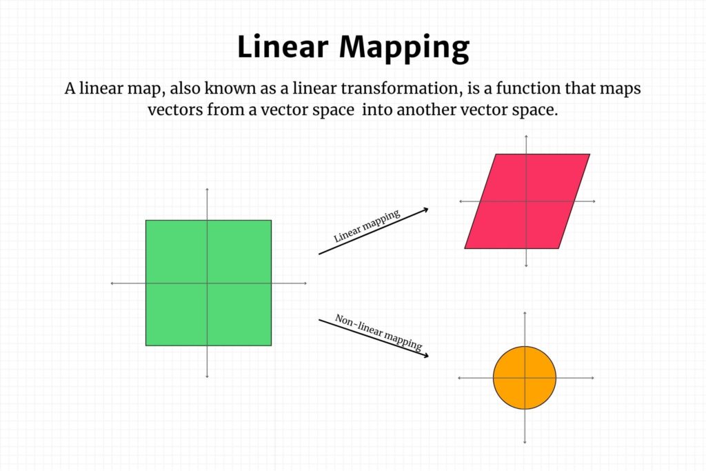
Linear mapping, also known as a linear transformation, is a fundamental concept in mathematics and a cornerstone in the field of data science and machine learning. At its core, a linear map is a function between two vector spaces that preserves the operations of addition and scalar multiplication. In simpler terms, it maintains the straightness of lines and the origin in vector spaces.
In this lesson, I’ll share with you the basic concepts of linear mapping and transformations. From isomorphisms to kernels of a linear map, you’ll gain insights into how linear mappings and transformations form the bedrock of numerous scientific and technological advancements.
As you explore further, you’ll discover how these concepts intricately intertwine with various branches of mathematics and data science, shaping the way we perceive and analyze the world around us.
Whether you’re unraveling the mysteries of chemical reactions or delving deep into the complexities of machine learning algorithms, understanding linear mappings and transformations will undoubtedly be your guiding light. Now, let’s get started.
Section 1: What is a Linear Map?
A linear map, also known as a linear transformation, is a function \( f: V \to W \) that maps vectors from a vector space \( V \) into another vector space \( W \). It satisfies two main properties, as shown below:
1. Additivity: \( f(\vec{u} + \vec{v}) = f(\vec{u}) + f(\vec{v}) \) for all \( \vec{u}, \vec{v} \in V \)
2. Homogeneity: \( f(c \vec{v}) = c f(\vec{v}) \) for all \( c \in \mathbb{R} \) and \( \vec{v} \in V \)
These properties ensure that the function \( f \) preserves the structure of the vector space. Given that a linear map \( f: V \to W \) obeys additivity and homogeneity, several derived properties naturally follow:
- Zero Mapping (\( f(\vec{0}) = \vec{0} \)): A linear map always maps the zero vector in \( V \) to the zero vector in \( W \).
- Scalar Distribution \( f(c_1 \vec{u} + c_2 \vec{v}) = c_1 f(\vec{u}) + c_2 f(\vec{v}) \): This property shows how scalars can be distributed across vectors before or after the transformation.
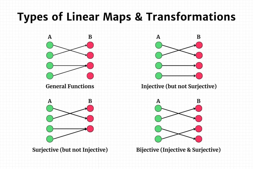
- Injectivity: A linear map is said to be injective if different vectors in \( V \) are mapped to different vectors in \( W \), a one-to-one map of sets. Formally, \( f(\vec{u}) = f(\vec{v}) \) implies \( \vec{u} = \vec{v} \).
- Surjectivity: A linear map is surjective if every vector in \( W \) is an image of some vector in \( V \).
- Bijectivity: A linear map is bijective if it is both injective and surjective, implying there exists an inverse function \( f^{-1}: W \to V \).
Section 2: Types of Linear Maps
Understanding the types of linear maps is pivotal for grasping how transformations can influence the structure and properties of vector spaces. In this section, we’ll delve into three main types of linear maps: bijective, injective, and surjective linear maps.
Bijective Linear Maps
A linear map \( f: V \to W \) is called bijective if it is both injective and surjective. This means that \( f \) uniquely maps every vector in \( V \) to a vector in \( W \) and covers the entire vector space \( W \).
- Injectivity: \( f(\vec{u}) = f(\vec{v}) \) implies \( \vec{u} = \vec{v} \)
- Surjectivity: For every \( \vec{w} \in W \), there exists a \( \vec{v} \in V \) such that \( f(\vec{v}) = \vec{w} \)
If a linear map is bijective, then it has an inverse \( f^{-1}: W \to V \) which is also a linear map. The existence of an inverse makes bijective linear maps extremely useful in algorithms requiring reversibility or undoing transformations.
Injective Linear Maps
An injective linear map, or one-to-one map, uniquely maps vectors from \( V \) to \( W \) without any overlaps. In formal terms, if \( f(\vec{u}) = f(\vec{v}) \), then \( \vec{u} = \vec{v} \).
- Zero Kernel: The kernel of an injective linear map contains only the zero vector, denoted as \( \text{ker}(f) = \{ \vec{0} \} \)
Injective maps are important in data science and machine learning for tasks such as dimensionality reduction, where we want to minimize information loss during the mapping.
Surjective Linear Maps
In contrast, a surjective linear map covers the entire vector space \( W \), meaning every vector in \( W \) is mapped from some vector in \( V \).
- Full Range: The range (or image) of \( f \) is equal to \( W \), mathematically expressed as \( \text{range}(f) = W \)
Surjective maps find applications in machine learning tasks like generating synthetic data and in algorithms that require full coverage of the output space.
Section 3: Isomorphisms
An isomorphism is a bijective linear map \( f: V \to W \) between two vector spaces \( V \) and \( W \) that has an inverse \( f^{-1}: W \to V \). Essentially, an isomorphism is a transformation that allows us to convert one vector space into another without losing any of the algebraic properties. It provides a one-to-one correspondence between the elements of \( V \) and \( W \), and is reversible.
Mathematically, an isomorphism \( f \) and its inverse \( f^{-1} \) satisfy:
- \( f(f^{-1}(\vec{w})) = \vec{w} \) for all \( \vec{w} \in W \)
- \( f^{-1}(f(\vec{v})) = \vec{v} \) for all \( \vec{v} \in V \)
Isomorphisms have a variety of applications in machine learning, some of which include:
- Feature Space Mapping: In support vector machines and kernel methods, isomorphisms can help in mapping the original feature space to a higher-dimensional space, making it easier to find a separating hyperplane.
- Data Preprocessing: When performing data normalization or other linear transformations, identifying an isomorphism ensures that we can revert the transformation without loss of information. This is particularly useful in exploratory data analysis and model interpretability.
- Optimization: Recognizing isomorphic structures can simplify complex optimization problems by reducing them to more manageable forms without altering the problem’s inherent characteristics.
Section 4: Homomorphisms
On the other hand, homomorphism is a structure-preserving map between two algebraic structures. In the context of linear algebra, it would mean a linear map \( f: V \to W \) between two vector spaces \( V \) and \( W \). The term “structure-preserving” indicates that vector addition and scalar multiplication in \( V \) are mirrored in \( W \) through \( f \).
Properties of Homomorphisms
Mathematically, a map \( f \) is a homomorphism if for all vectors \( \vec{u}, \vec{v} \in V \) and all scalars \( c \), the following properties hold:
- \( f(\vec{u} + \vec{v}) = f(\vec{u}) + f(\vec{v}) \)
- \( f(c \vec{u}) = c f(\vec{u}) \)
Both homomorphisms and isomorphisms are structure-preserving maps, but they’re not identical in their roles:
- Isomorphism: An isomorphism is a special case of a homomorphism that is bijective (i.e., injective and surjective), which means it has a two-way, reversible relationship between \( V \) and \( W \).
- Homomorphism: A homomorphism might be neither injective nor surjective, which implies it may not be reversible. In other words, all isomorphisms are homomorphisms, but not all homomorphisms are isomorphisms.
Applications of Homomorphisms
The concept of homomorphism plays a key role in various machine learning scenarios:
- Dimensionality Reduction: Principal Component Analysis (PCA) can be thought of as a homomorphism where the original data vectors are linearly mapped to a lower-dimensional space. This transformation is not bijective, hence it’s a homomorphism but not an isomorphism.
- Data Transformation: When we perform data normalization, we’re essentially applying a homomorphism that scales and translates the data vectors. Though structure-preserving, these transformations might not be reversible if some information is lost or generalized.
- Feature Engineering: Creating polynomial features from linear features in regression models is another example of a homomorphic transformation that enables linear models to capture nonlinear relationships.
Section 5: Kernel of a Linear Map
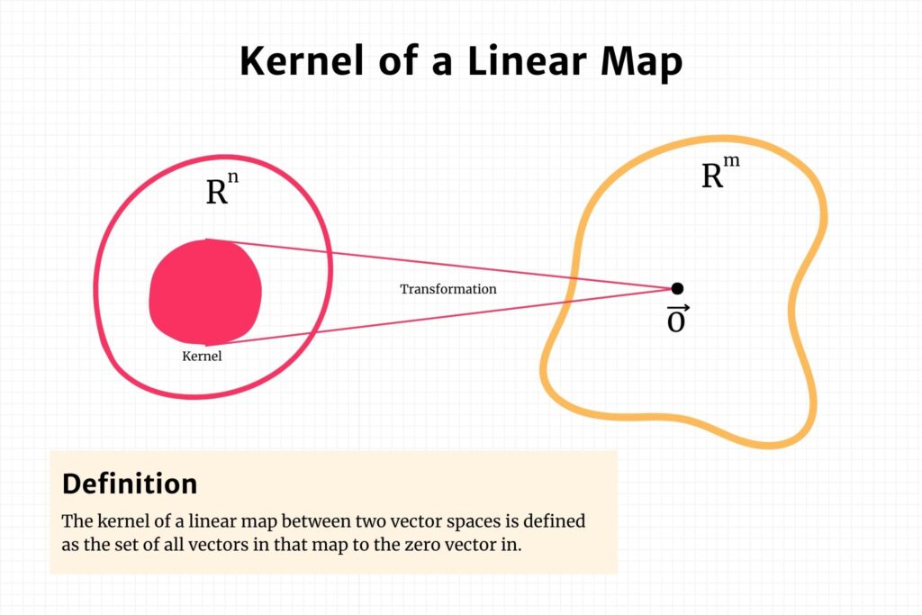
The kernel of a linear map \( f: V \to W \) between two vector spaces \( V \) and \( W \) is defined as the set of all vectors in \( V \) that map to the zero vector in \( W \). Mathematically, it can be expressed as:
\[\text{Ker}(f) = \{ \vec{v} \in V | f(\vec{v})=0\} = f^{-1}(0) \]
The kernel is a subspace of the domain \( V \) and offers insights into the ‘nullity’ of the transformation, essentially telling us the dimension of the space that gets “collapsed” to the zero vector in \( W \).
Computing the kernel of a linear map usually involves finding the solution to the equation \(f(\vec{v})=0\} = f^{-1}(0)\). Here are some computational techniques:
- Matrix Representation: If \( f \) can be represented as a matrix \( A \), finding the kernel is equivalent to solving the homogeneous equation \( A\vec{x} = \vec{0} \).
- Row Reduction: Employ Gaussian elimination to row-reduce the augmented matrix \([A|\vec{0}]\) to its row-reduced echelon form. The solutions to the resulting system will constitute the kernel.
- Eigenvalue Method: In some cases, especially when \( A \) is a square matrix, finding the eigenvalues and eigenvectors can aid in computing the kernel. If 0 is an eigenvalue, its corresponding eigenvectors will form a basis for the kernel.
- Computational Software: Software packages like NumPy, MATLAB, and specialized libraries in programming languages can efficiently calculate the kernel, especially for large-scale problems common in machine learning applications.
To sum up, the kernel of a linear map is not just a mathematical curiosity; it’s a crucial concept that finds numerous applications in data science and machine learning. Understanding its properties and how to compute it gives you a powerful tool for dissecting the intricacies of linear transformations.
Conclusion
In the realm of machine learning and data science, the importance of understanding linear maps and transformations cannot be overstated. We’ve journeyed through a comprehensive exploration of this subject, touching upon fundamental definitions, types of linear maps, and key concepts like isomorphisms, homomorphisms, and the kernel of a linear map. Not only did we delve into the mathematical underpinnings, but we also elucidated the crucial role these constructs play in various machine learning algorithms and real-world applications.
- What is a Linear Map: A foundational mathematical structure that encapsulates how vectors in one space are transformed into another.
- Types of Linear Maps: Understanding injective, surjective, and bijective maps adds nuance to how transformations can be categorized.
- Isomorphisms and Homomorphisms: Special types of linear maps that have unique properties and applications in machine learning.
- Kernel of a Linear Map: A significant concept that offers insights into the ‘null space’ of a transformation.
Linear algebra serves as the bedrock upon which many machine learning algorithms are built. Thus, mastery over concepts like linear maps and transformations not only fortifies your foundational knowledge but also provides you with the analytical tools to innovate and excel in this burgeoning field. The landscape is ever-evolving, and staying ahead necessitates a commitment to continuous learning.
By seizing the opportunity to further explore these topics, you are taking a significant step toward not just being a participant in the world of machine learning, but also being a contributor to its ever-expanding frontier.
Should you have more questions or require further clarification on any topic covered in this article, feel free to reach out. Your journey in mastering linear algebra in the context of machine learning is a voyage worth undertaking.