Linear Combinations of Vectors & Spans

If you’ve ever dabbled in machine learning or data science, you’ve probably encountered terms that made your head spin. Linear algebra, vectors, scalars—these aren’t just buzzwords; they’re the backbone of algorithms and models that make sense of massive amounts of data. Among these, one term you’ll often come across is “linear combinations.” In its simplest form, a linear combination lets you construct a new vector by adding together existing vectors, scaled by some numbers. It’s a little like cooking; you mix specific amounts of ingredients to create a new dish.

But why does it matter? Well, understanding linear combinations and related concepts like “spans” and “basis sets” is like learning the grammar of machine learning. You’ll find these ideas embedded in popular algorithms like Support Vector Machines and Principal Component Analysis. So, whether you’re just starting your journey in machine learning or a seasoned pro looking for a refresher, you’re in the right place.

In this article, you’ll:

• Learn what linear combinations are and see them in action mathematically.
• Understand how the idea of a “span” evolves from linear combinations and what role it plays in data science.
• Discover why knowing about basis sets can be a game-changer in your machine learning projects.

So buckle up. We’re about to dive into a topic that may seem abstract at first, but by the end, you’ll see how grounded it is in the world of machine learning and data science.

Section 1: What are Linear Combinations?

Understanding linear combinations requires a foundational grasp of two key mathematical objects: vectors and scalars. While these terms may sound technical, they have practical importance in machine learning and data science. Let’s unpack what they are.

Defining Vectors & Scalars

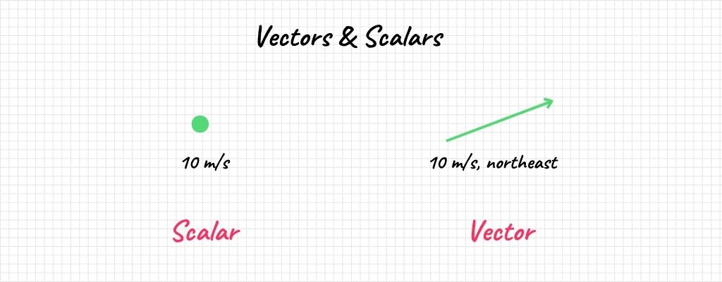
Vectors are a staple in the world of machine learning. Think of them as arrows pointing in a certain direction, with a specific length. They’re not just abstract entities; they have real-world applications. For example, in a recommendation algorithm, each vector could represent a user or an item like a movie or a book. The “direction” they point in could signify user preferences or item attributes.

Mathematically, a vector in a 2D space is represented as \( \textbf{v} = [v_1, v_2] \), and its extension to higher dimensions follows a similar structure. In machine learning, we often deal with vectors with hundreds or even thousands of dimensions, each representing a specific feature of the data.

Now, if vectors are the ingredients in our “recipe,” then scalars are the portions. A scalar is simply a number that scales a vector—makes it longer or shorter without affecting its direction. In the formula for a linear combination,

\[\textbf{v} = c_1\textbf{a}_1 + c_2\textbf{a}_2 + \cdots + c_n\textbf{a}_n\]

each \( c_n \) is a scalar that alters the size of the vector \( \textbf{a}_n \).

Vectors and scalars may be basic building blocks, but their roles are pivotal. They lay the groundwork for more complex concepts like linear combinations, which we’ll explore in detail in the subsequent sections.

Mathematical Expression of Linear Combinations

Having established the significance of vectors and scalars, it’s now time to delve into the formal mathematics of linear combinations. The concept itself is eloquently captured by a simple yet powerful formula:

\[\textbf{v} = c_1\textbf{a}_1 + c_2\textbf{a}_2 + \cdots + c_n\textbf{a}_n\]

Here, \(\textbf{v}\) represents the resulting vector we get when we combine vectors \( \textbf{a}_1, \textbf{a}_2, \ldots, \textbf{a}_n \) using scalars \( c_1, c_2, \ldots, c_n \) as multipliers.

Let’s break down what each component means:

• Vector \( \textbf{v} \): This is the new vector formed by the linear combination. It could represent anything from a point in a Cartesian plane to a complex structure in a machine learning model.
• Vectors \( \textbf{a}_1, \textbf{a}_2, \ldots, \textbf{a}_n \): These are the existing vectors you’re starting with. Each one could signify a different attribute or feature in a data set. In a 3D space, they can be visualized as arrows pointing in different directions.
• Scalars \( c_1, c_2, \ldots, c_n \): These numbers serve as the ‘coefficients’ or multipliers for each vector. They scale the vectors, either stretching or shrinking them, to contribute a certain amount to the resulting vector \( \textbf{v} \).

The beauty of this formula lies in its flexibility. In the context of machine learning, it’s often used implicitly within algorithms to make predictions, classify data, or even reduce dimensions.

By understanding how to express linear combinations mathematically, you’re setting yourself up for a deeper comprehension of numerous algorithms and techniques in machine learning and data science.

Geometric Interpretation

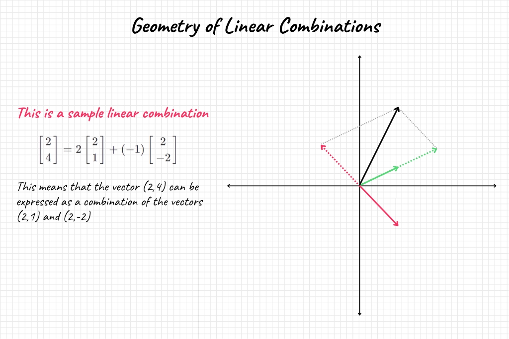
Mathematics becomes remarkably intuitive when we can visualize it. The concept of linear combinations is no different. Imagine you’re given two vectors, \( \textbf{a} \) and \( \textbf{b} \), in a 2D space. These vectors can be thought of as arrows originating from the origin and pointing to some point in the plane. 

When you perform a linear combination, you’re essentially “walking” along these vectors. Scaling the vector \( \textbf{a} \) by \( c_1 \) is like stretching or compressing the arrow, and then adding it to \( c_2 \textbf{b} \) is similar to “walking” along \( \textbf{b} \) after you’ve “walked” along \( \textbf{a} \). The point where you end up is the tip of the resulting vector \( \textbf{v} \).

In 3D or higher dimensions, the concept holds. You’re effectively navigating through a multi-dimensional “landscape” by walking along different vectors, each scaled by a specific scalar. This idea is often employed in machine learning to navigate the high-dimensional spaces that data can exist in.

Special Cases of Linear Combinations

• Zero Vector: The zero vector is a particularly interesting case. It’s a vector where all components are zero, represented as \( \textbf{0} = [0, 0, \ldots, 0] \). The zero vector is often the “result” when all the scalars in a linear combination are zero, i.e.,

\[\textbf{0} = 0\textbf{a}_1 + 0\textbf{a}_2 + \cdots + 0\textbf{a}_n\]

• Unit Vectors: Unit vectors are vectors of length 1 and often serve as the “building blocks” in the realm of linear algebra. The most common unit vectors are \( \textbf{i} \), \( \textbf{j} \), and \( \textbf{k} \) in 3D, which point along the x, y, and z-axes, respectively. Linear combinations of unit vectors can form any other vector in the space as shown in the equation below.Unit vectors are especially important in algorithms like Principal Component Analysis (PCA), where the goal is to find the unit vectors that maximize variance in a dataset.

\[\textbf{v} = v_x\textbf{i} + v_y\textbf{j} + v_z\textbf{k}\]

Understanding the geometric nuances and the special cases of linear combinations enriches your grasp of how these fundamental concepts come alive in machine learning and data science. This sets the stage for more advanced topics, like spans and basis sets, which we’ll explore next.

Section 2: Spans

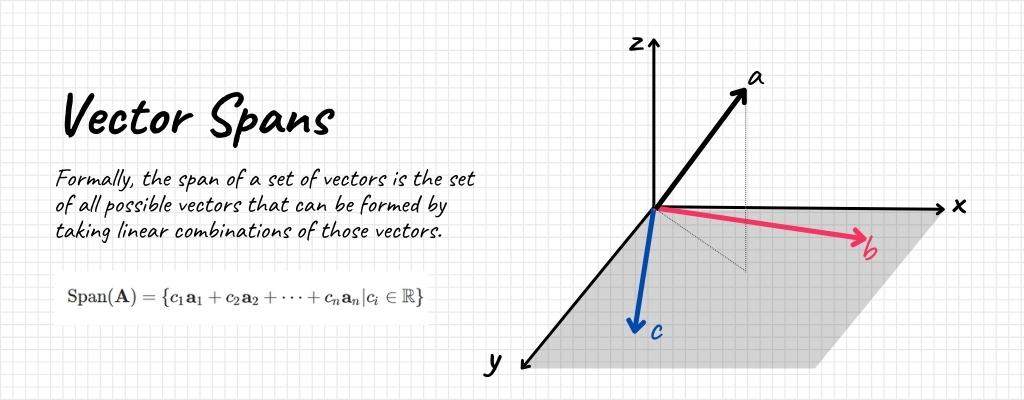
A span can be thought of as the “scope” or “reach” of a set of vectors. Formally, the span of a set of vectors is the set of all possible vectors that can be formed by taking linear combinations of those vectors. In simpler terms, if you are given a few vectors, the span is basically all the places you can get to by scaling and adding those vectors together.

Span in the Context of Linear Combinations

As mentioned previously, the concept of a span is inherently tied to that of a linear combination. If you are given a set of vectors \( \textbf{A} = \{ \textbf{a}_1, \textbf{a}_2, \ldots, \textbf{a}_n \} \), then the span of \( \textbf{A} \) is all the vectors you can create by taking linear combinations of vectors in \( \textbf{A} \). Mathematically, this is expressed as:

\[\text{Span}(\textbf{A}) = \{ c_1\textbf{a}_1 + c_2\textbf{a}_2 + \cdots + c_n\textbf{a}_n | c_i \in \mathbb{R} \}\]

Here, \( c_i \in \mathbb{R} \) indicates that the coefficients can be any real numbers, making the span a very versatile concept. In machine learning, understanding the span of your feature vectors can offer insights into the complexity and dimensionality of your problem space.

Degrees of Freedom

The idea of a “degree of freedom” can be thought of as how much “wiggle room” or how many options you have in a given situation. In the context of spans, the degrees of freedom relate to how much of the vector space your set of vectors can “cover.”

For instance, if you have two non-parallel vectors in a 2D plane, their span is the entire plane—you can reach any point in the plane by scaling and adding these vectors. Therefore, you have 2 degrees of freedom in this case. However, if both vectors are parallel (or one is a zero vector), you can only move along that line. Thus, you have just 1 degree of freedom.

Understanding degrees of freedom is pivotal when dealing with machine learning models. Too many degrees of freedom might lead to overfitting, where your model is so flexible that it performs poorly on unseen data. On the flip side, too few could result in underfitting, where the model can’t capture the underlying pattern in the data.

Section 3: Basis Sets

A basis of a vector space is a set of linearly independent vectors that span the entire vector space. Linearly independent means that no vector in the set can be expressed as a linear combination of the other vectors. 

In essence, a basis gives you the “minimum set of directions” needed to get to any point in the space. Formally, for a set of vectors \( \textbf{B} = \{ \textbf{b}_1, \textbf{b}_2, \ldots, \textbf{b}_n \} \) to be a basis, two conditions must be met:

1. The vectors must be linearly independent.
2. The span of \( \textbf{B} \) must be equal to the vector space \( V \), i.e., \( \text{Span}(\textbf{B}) = V \).

Orthogonal and Orthonormal Basis

An orthogonal basis is a set of vectors that are not only linearly independent but also perpendicular to each other. If these vectors are also of unit length, then the basis is called orthonormal. 

\[\textbf{b}_i \cdot \textbf{b}_j = \begin{cases}  1, & \text{if \( i = j \)} \\  0, & \text{otherwise}\end{cases}\]

Orthogonal and orthonormal bases have significant computational advantages, particularly in numerical calculations, because the vectors are decorrelated. They simplify many operations like projections and rotations.

Section 4: Application in Machine Learning

SVM & Linear Combinations

Support Vector Machines (SVM) are a class of supervised learning algorithms used for classification or regression tasks. One of the key ideas behind SVM is finding the hyperplane that best separates different classes in a high-dimensional space. Linear combinations play a crucial role here.

Given a set of vectors \( \textbf{x}_1, \textbf{x}_2, \ldots, \textbf{x}_n \), the optimal hyperplane is determined by a linear combination of these vectors. The equation of the hyperplane in SVM can be represented as:

\[\textbf{w} \cdot \textbf{x} + b = 0\]

where \( \textbf{w} \) is a weight vector, which itself is a linear combination of the input vectors, and \( b \) is the bias term. Understanding linear combinations allows you to grasp how SVM finds the most optimal separating hyperplane.

PCA & Dimensionality Reduction

Principal Component Analysis (PCA) is a dimensionality reduction technique that identifies the axes (basis vectors) along which the data varies the most. Essentially, it finds a new basis set for your data, where the vectors are sorted by the amount of variance they capture. 

The primary components in PCA can be obtained through eigenvalue decomposition of the data’s covariance matrix \( \Sigma \):

\[\Sigma = \textbf{V} \Lambda \textbf{V}^T\]

Here, \( \Lambda \) is a diagonal matrix containing eigenvalues, and \( \textbf{V} \) contains the corresponding eigenvectors. These eigenvectors form the new basis set for the data.

Other Advanced Topics

• Tensor Decompositions: In more advanced machine learning algorithms, particularly in the context of deep learning, tensors (multi-dimensional arrays) are often used. Tensor decompositions, such as CANDECOMP/PARAFAC (CP) or Tucker decomposition, generalize matrix factorization techniques to tensors and can be useful for data compression, noise reduction, or feature extraction.
• Manifold Learning: Manifold learning techniques like t-SNE, Isomap, or UMAP aim to find a low-dimensional basis (or manifold) that captures the high-dimensional data’s intrinsic structure. While these techniques go beyond linear combinations and spans, understanding these basic concepts can provide the foundation needed to grasp more advanced topics like manifold learning.

These are just a few examples of how the concepts of linear combinations, spans, and basis sets are directly applied in machine learning algorithms. This understanding allows data scientists to not just implement these algorithms but also to optimize and even innovate on existing techniques.

Section 5: Refresh and Reinforce

Even professionals can sometimes overlook some of the more advanced theorems or techniques. Here are a few you might want to refresh:

Gram-Schmidt Orthogonalization: This process takes a set of vectors and produces an orthogonal or orthonormal basis. While this may seem rudimentary, it’s crucial for algorithms like QR decomposition. The Gram-Schmidt process starts with an arbitrary basis and refines it iteratively:

\[\textbf{u}_k = \textbf{a}_k – \sum_{j=1}^{k-1} \text{proj}_{\textbf{u}_j} \textbf{a}_k\]

Singular Value Decomposition (SVD): Used in machine learning for dimensionality reduction and noise reduction, SVD is often glossed over. It can decompose any given matrix into three other matrices and gives insights into the “most important” dimensions in a dataset.

\[A = U \Sigma V^*\]

Jordan Normal Form: Especially useful in the context of differential equations and dynamical systems, the Jordan normal form generalizes the concept of diagonalization. It’s a way to simplify matrix exponentiation and is crucial in control theory.

\[A = PJP^{-1}\]

Spectral Clustering: This advanced technique is used in graph-based clustering and leverages the eigenvalues of the Laplacian matrix of the graph. Understanding the underlying linear algebra is critical for tuning and understanding this algorithm.

\[L = D – A\]

Conclusion

In this comprehensive guide, we’ve walked through the essential mathematical concepts of linear combinations of vectors, spans, and basis sets. For those new to machine learning, these topics offer a solid foundation in understanding how algorithms work beneath the surface. For seasoned professionals, revisiting these principles can illuminate aspects of optimization, dimensionality reduction, and various machine learning algorithms.

Key Takeaways

1. Linear Combinations: We understood that a linear combination involves multiplying vectors by scalars and adding them. The formula \( \textbf{v} = c_1\textbf{a}_1 + c_2\textbf{a}_2 + \cdots + c_n\textbf{a}_n \) summarizes this elegantly.
2. Spans: The span of a set of vectors provides you with the “reach” within the vector space. It can be expressed as \( \text{Span}(\textbf{A}) = \{ c_1\textbf{a}_1 + c_2\textbf{a}_2 + \cdots + c_n\textbf{a}_n | c_i \in \mathbb{R} \} \).
3. Basis Sets: We learned that basis sets are pivotal in simplifying complex vector spaces. An orthogonal or orthonormal basis set can further simplify calculations and are essential in algorithms like PCA.
4. Applications in Machine Learning: From SVM to PCA, linear algebra plays a crucial role. Understanding these fundamental concepts can significantly benefit your grasp of machine learning algorithms.

Future Applications and Next Steps

1. Deep Learning: As you delve deeper into neural networks, you’ll find that understanding the intricacies of vector spaces can drastically improve your models.
2. Quantum Computing: With the advent of quantum algorithms, linear algebra will only become more crucial. Concepts like superposition are direct extensions of our understanding of vector spaces.
3. Data Science Projects: You can now apply these concepts to real-world data science projects. Whether it’s optimizing a recommendation engine or simplifying a complex dataset using PCA, your enhanced understanding of linear algebra will be incredibly beneficial.
4. Continual Learning: The field is continuously evolving. Advanced topics like tensor decompositions and manifold learning are excellent areas for further study and can be directly applied in machine learning and data analytics.

To truly cement these concepts, consider applying them in your machine learning projects or exploring further through academic papers and advanced courses. You’ll find that a solid grounding in linear algebra not only makes complex topics more accessible but also opens the door to innovative solutions and approaches in your data science journey.

And with that, we wrap up our extensive look into linear combinations, spans, and basis sets in the context of machine learning. Whether you’re a novice or a seasoned professional, understanding these core mathematical concepts will undoubtedly enhance your expertise in the field.